Article abstract
Article abstract
Many pathogens reside in environmental reservoirs within which they can reproduce and from which they can infect hosts. These facultative pathogens experience different selective pressures in host-associated environments and reservoir environments. Heterogeneous selective pressures have the potential to influence the virulence evolution of these pathogens. Previous research has examined how environmental transmission influences the selective pressures shaping the virulence of pathogens that cannot reproduce in environmental reservoirs, yet many pathogens of humans, crop plants, and livestock can reproduce in these environments. We build on this work to examine how reproduction in reservoirs influences disease dynamics and virulence evolution in a simple facultative pathogen model. We use adaptive dynamics to examine the evolutionary dynamics of facultative pathogens under potential trade-offs between transmission and virulence, shedding and virulence, and reservoir persistence and virulence. We then perform critical function analysis to generalize the results independent of specific trade-off assumptions. We determine that diverse virulence strategies, sometimes resulting from evolutionary bistability or evolutionary branching conditions, are expected for facultative pathogens. Our findings motivate research establishing which trade-offs most strongly influence the virulence evolution of facultative pathogens.
Introduction
Introduction
This file presents the codes used to generate the figures presented in the accompanying article (Pandey, A., Mideo, N., & Platt, T. G. (2021). Virulence evolution of pathogens that can grow in reservoir environments. The American Naturalist). Here we explore the epidemiological and evolutionary outcomes for a simple facultative pathogen model: =b-βSI--dS=βSI+-(d+ρ+α)S=θI-σP+rP1- (1)The susceptible hosts (S) are born at a constant rate (b) and die at a per capita rate (d), with direct infection following mass action incidence with rate constant β. The recovery rate is ρ, and we assume lifelong immunity once the host is recovered. The contact rate between susceptible hosts and pathogens in the environmental reservoir is an increasing but saturating function of P, described by ϕP/(P+τ). The term γ represents the probability of environmental transmission on contact with pathogens in the reservoir. Free-living pathogen population dynamics depend on shedding from infected hosts at rate θ, death of free-living pathogen propagules at rate σ, and density-dependent (specifically, logistic) reproduction of pathogen propagules at per capita rate r. K represents the carrying capacity in the reservoir.
dS
dt
γSϕP
(τ+P)
dI
dt
γSϕP
(τ+P)
dP
dt
P
K
Figure 2a. Differences in threshold parameters: R0d vs λ
Figure 2a. Differences in threshold parameters: vs λ
R
0d
λ is the demographic reproduction number and is derived from the Jacobian of Infected- Free-living pathogen system (equation 1). R0d represents the number of secondary infections that arise from a single infected individual before the pathogen reproduces in the reservoir. The code below shows the effect of virulence (α) and pathogen growth rate in environment (r) on these two metrics through a contour plot. Disease spreads in population if either of R0d and λ is greater than 1. Please refer to the paper and its appendix section for more details on these metrics.
λ is the demographic reproduction number and is derived from the Jacobian of Infected- Free-living pathogen system (equation 1). represents the number of secondary infections that arise from a single infected individual before the pathogen reproduces in the reservoir. The code below shows the effect of virulence (α) and pathogen growth rate in environment (r) on these two metrics through a contour plot. Disease spreads in population if either of and λ is greater than 1. Please refer to the paper and its appendix section for more details on these metrics.
R
0d
R
0d
Clear["Global`*"](* Parameter values *)Pars={b1,d 0.2,γ0.1,σ0.5,θ0.1,β0.1};(* Define λ *)λ=1/2(β*b/(d*(d+α))+r/σ+Sqrt[(β*b/(d*(d+α))-r/σ)^2+4*γ*b/(d*σ)*θ/(d+α)] )/.Pars;(* Define R0 *)R0d=β*b/(d*(d+α))+γ*b/(d*σ)*θ/(d+α) /.Pars;Show[ ContourPlot[ λ,{α,0,2},{r,0,1}, Contours{1}, RegionFunctionFunction[ {α,r,R0d},R0d>1 ], ContourShading{Darker[Orange,.008]} ], ContourPlot[ λ,{α,0,2},{r,0,1}, Contours{1}, RegionFunctionFunction[ {α,r,R0d},R0d<1 ], ContourShading{Lighter[Orange,1/2]} ], ContourPlot[ R0d,{α,0,2},{r,0,1}, Contours{1}, RegionFunctionFunction[ {α,r,R0d},R0d>1 ], ContourShading{Darker[Orange,1/5]} ], FrameLabel{"Virulence (α)","Free-living pathogen birth rate (r)"}, Frame{True,True,False,False}, FrameStyleDirective[Black,15], FrameTicks{{0.5,1.0,1.5,2.0},{0.2,0.4,0.6,0.8,1.0}}, LabelStyleDirective[Black,15], Epilog Text[Style["λ > 1",Medium],{0.25,0.6}], Text[Style[Subscript[R,"0d"]>1,Medium],{0.25,0.55}], Text[Style["λ > 1",Medium],{1,0.6}], Text[Style[Subscript[R,"0d"]<1,Medium],{1,0.55}], Text[Style["λ < 1",Medium],{1,0.25}], Text[Style[Subscript[R,"0d"]<1,Medium],{1,0.2}] ]
Out[]=
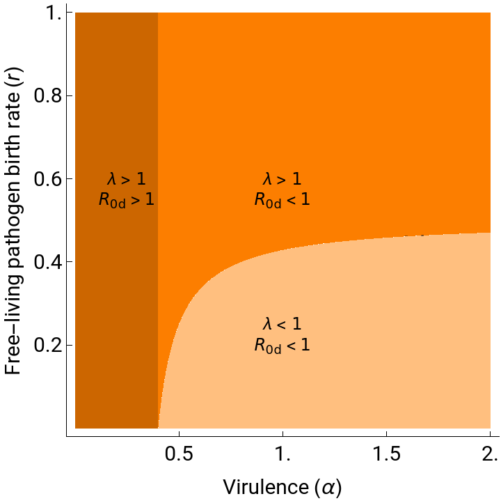
Figure 2b. Effect of free-living pathogens and reservoir carrying capacity in endemic disease prevalence
Figure 2b. Effect of free-living pathogens and reservoir carrying capacity in endemic disease prevalence
Clear["Global`*"](*Parameter values *)Pars={b1,γ 0.3,d 0.2,ρ 0,β0.01,θ0.1,σ0.1,α0.3};(* System of equations *)dS= b-(β*S[t]*Inf[t])-(γ*S[t]*(P[t]/(P[t]+1)))-(d*S[t]) /.Pars;dI=(β*S[t]*Inf[t])+(γ*S[t]*(P[t]/(P[t]+1)))-(d+ρ+α)*Inf[t] /.Pars;dP=(θ*Inf[t])-σ P[t]+r P[t] (1-P[t]/Ka) /.Pars;(* Equilibrium solutions *)sol2=Solve[{dS0,dI0,dP0},{S[t],Inf[t],P[t]}];(* Plotting disease prevalence at endemic equilibrium solution *)ContourPlot[ {Inf[t]/(S[t]+Inf[t])}/.sol2[[5]], {r,0.1,0.5}, {Ka,2,20}, FrameLabel{"Growth rate (r)","Carrying capacity (K)"}, LabelStyleDirective[Black,15], FrameStyleDirective[Black,15], FrameTicks {{5,10,15,20},None},{{0.1,0.2,0.3,0.4,0.5},None} , PlotLegendsBarLegend[Automatic,LegendMarkerSize140,LegendFunction"Frame",LegendLabel->"Prevalence"], ColorFunctionGrayLevel ]
Out[]=
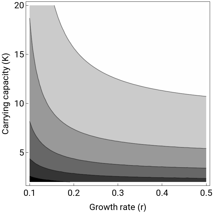
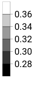
Fig 3. PIPs under transmission-virulence trade-off
Fig 3. PIPs under transmission-virulence trade-off
Here we generate the pairwise-invasibility-plot (PIP) to show the effect of transmission-virulence trade-off. You can change the value of h to change the strength of trade-off.
Fig 4. PIPs for transmission-virulence + shedding-virulence trade-offs
Fig 4. PIPs for transmission-virulence + shedding-virulence trade-offs
Here we generate the pairwise - invasibility - plot (PIP) to show the combined effect of transmission - virulence and shedding - virulence trade - offs . The procedures are similar to figure 3.
Fig 5a. Persistence-virulence trade-off
Fig 5a. Persistence-virulence trade-off
Fig 6a. Bifurcation diagram under multiple trade-offs with changing u (persistence-virulence strength)
Fig 6a. Bifurcation diagram under multiple trade-offs with changing u (persistence-virulence strength)
In this section, we generate the so called bifurcation diagrams that represent different types of singular strategies. Singular strategies are those strategy values where the fitness gradient vanishes. The techniques of finding different singular strategies are given as comments with the code below. Here, we look at the effect of changing persistence-virulence trade-off by changing the parameter u.
Note: This section is computationally intensive and generates large outputs (> 1 GB).
Fig 6b-d. PIPs for multiple trade-offs
Fig 6b-d. PIPs for multiple trade-offs
Here, we use persistence-virulence trade-off in addition to the shedding-virulence and transmission-virulence trade-offs. Change the parameters (e.g. u for changing persistence-virulence trade-off) as mentioned in the main text to get different PIPs.
Fig 7a. Bifurcation diagram with varying reservoir carrying capacity
Fig 7a. Bifurcation diagram with varying reservoir carrying capacity
Similar to the section 6a, we now generate the bifurcation diagram where we look at the effect of reservoir carrying capacity on different singular strategies.
Note: This section is computationally intensive and generates large outputs (> 1 GB).
Fig 7b-d. PIPs with varying reservoir carrying capacity
Fig 7b-d. PIPs with varying reservoir carrying capacity
This code generates PIPs with different reservoir carrying capacity. Just change the value of Ka in the code to generate different PIPs.
Fig 8b. Evolutionary branching point
Fig 8b. Evolutionary branching point
This section shows a special PIP with evolutionary branching point. These are convergence stable but evolutionary stable points.
Fig 8 a. Evolutionary branching point
Fig 8 a. Evolutionary branching point
This part shows the critical function analysis. This shows family of curves for critical function with different initial conditions. Then we can imagine trade-off of any shapes. The points where the assumed trade-off is tangent to the critical function represents singular points. The geometry of trade-off and critical function at the tangent point can determine different types of singular points. See the main text for more details.