In this notebook, we formalize the mathematical framework of Lie theory, using 3D rotations as a driving example. While we have previously applied Lie theory to rotational dynamics, we took many mathematical facts on faith. Here, in a structured, cheat-sheet style, we derive everything, proceeding from the central concept, the Lie algebra, to the and rotational Lie groups, which emerge naturally via representation theory.
(2)
SO(3)
SU(2)
In short, this notebook serves as a physics-centric introduction to Lie theory, showing techniques that generalize far beyond 3D rotations.
Preliminaries
Preliminaries
Lie Ontology
Lie Ontology
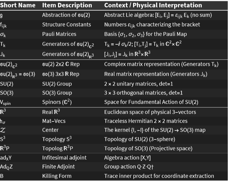
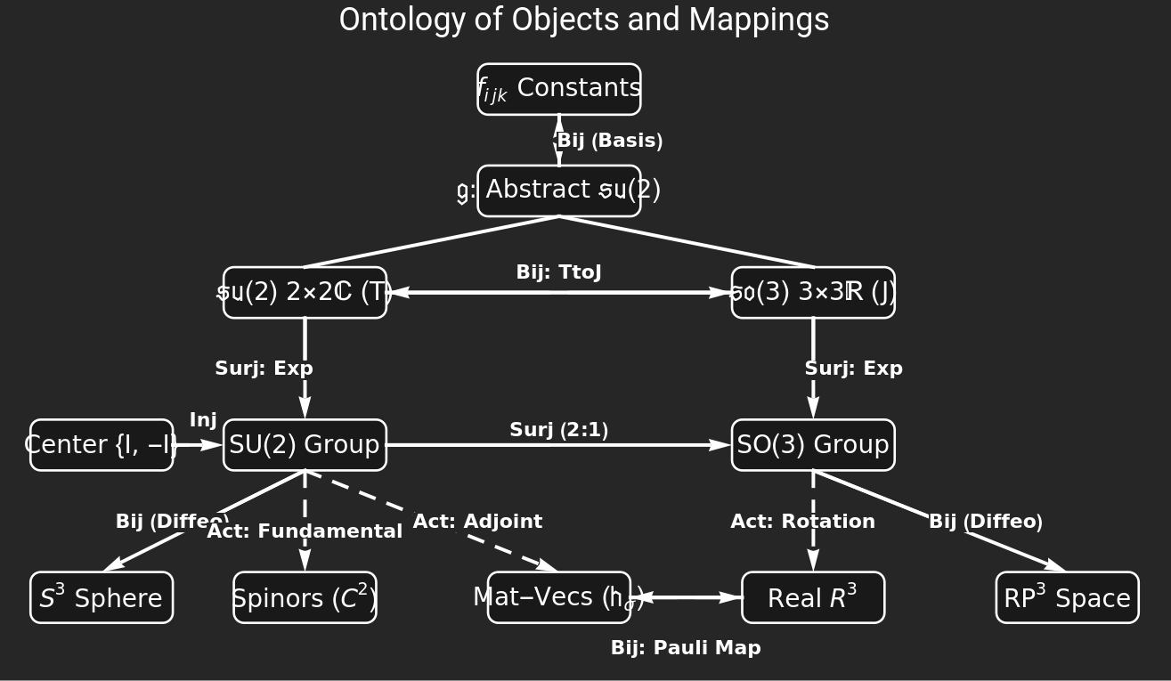
One of the most important applications of Lie theory is for 3D rotations. In two earlier notebooks, for Classical Mechanics and SU(2) for Classical Mechanics, we showed how to solve dynamical problems via geodesics in the Lie groups and , with metric tensors composed of kinetic energies. We demonstrated the superiority of in avoiding the gimbal lock in the Euler-angle parameterization of , by honoring the intrinsic, simply connected topology of the configuration space of rotations. In those notebooks, we developed just enough of the mathematical theory to assure the application, in a “just-in-time” style. This style left us with several pieces of theory “on the table.” Here, we organize those pieces and fit them together in a tidy structure that’s easy to understand, to remember, and to be creative with. We first give an inventory of the objects and mappings in the theory, and then present a diagram linking them together. In the rest of the notebook, we work out the details formally, machine-checked by Wolfram.
SO(3)
SU(2)
SU(2)
SO(3)
Object Inventory
Object Inventory
The “big picture” for rotations is that we can represent the abstract Lie algebra of in at least two ways. One of them leads us to and its troubles with gimbal lock (via the non-trivial fundamental group (SO(3))=), the other to with no such troubles and, thus, a virtuous slippery slope to quantum theory.
(2)
SO(3)
π
1
2
SU(2)
◼
Representation is a formal notion: mapping the abstraction to matrices. Representation theory itself is an immense topic. Here we need just a basic understanding.
◼
Abstractly, a Lie algebra is a vector space with a Lie bracket operation, , that satisfies the Jacobi identity, . In a matrix representation, the Lie bracket is the matrix commutator .
[A,B]
[A,[B,C]]+[C,[A,B]]+[B,[C,A]]=0
[A,B]=A·B-B·A
The abstract algebra, , for 3D rotations is characterized by its its specific structure constants. In general, the structure constants of any Lie algebra-qua-vector-space are the Lie bracket applied to a choice of basis vectors: (sum over ). The specific structure constants for rotations are , the fully antisymmetric Levi-Civita tensor, where , , are in . These structure constants model the cross product, familiar from elementary physics as the primary tool for describing rotation. In the real domain, these structure constants imply the generators . In the complex domain, they imply the generators . The corresponding Lie groups follow via the exponential map.
f
ijk
,=
E
i
E
j
f
ijk
E
k
k
ϵ
ijk
i
j
k
{1,2,3}
J
k
T
k
◼
A Lie group is both a group and a differentiable manifold. As a manifold, it enjoys parameterization by coordinate charts that must be differentiable where they overlap. As a group, its elements describe linear transformations of other objects, spinors and mat-vecs in our running example.
◼
The adjoint action, is linear in .
Q·v·Q
v
The double-covering of by follows from the topology of their respective manifolds. is diffeomorphic to the real projective space , visualized as the 3-sphere , where every point is identified with its antipode, . is not simply connected because any closed loop in that includes both and , the same point in , is a closed loop in that cannot be shrunk to zero size without “tearing”. In contrast, is diffeomorphic to . This space is simply connected because any closed path can be shrunk to zero size.
SO(3)
SU(2)
SO(3)
3
P
3
S
(q∼(-q))
3
P
3
S
q
-q
3
P
3
P
SU(2)
3
S
◼
3
S
q≡(,,,)
q
0
q
1
q
2
q
3
4
+++=1
2
q
0
2
q
1
2
q
2
2
q
3
◼
In , points are actually pairs of elements of .
3
P
(q,-q)
4
The elements of each group describe linear transformations of geometric objects that are not elements of the group. Concretely, we represent the linear transformations as matrices that operate on -vectors. We represent by real rotation matrices that act on real 3-vectors. We represent by complex matrices, isomorphic to unit quaternions, that act on spinors in = and on complex, , traceless, Hermitian matrices (mat-vecs in ) that represent real 3-vectors.
n×n
n
SO(3)
3×3
SU(2)
2×2
V
spin
2
2×2
σ
◼
The algebra is isomorphic to the pure imaginary quaternions, .
(2)
(0,,,)
q
1
q
2
q
3
Finally, we introduce some notation, and , for actions in the Lie algebra and the Lie Group respectively, and the Killing form for extracting components of members of the Lie groups.
ad
X
Ad
Q
Out[]=
Mapping Inventory
Mapping Inventory
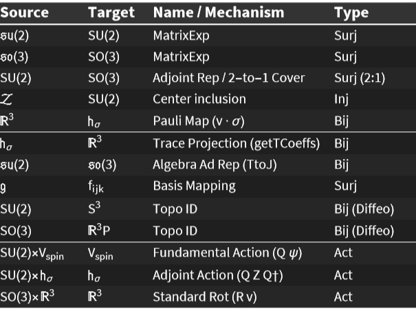
Here we list, non-exhaustively, various mappings amongst the objects above. MatrixExp takes us from a representation of an element of a Lie algebra to a representation of an element of a Lie Group. This is a surjection in that multiple inputs can produce the same output. Not listed is the inverse, MatrixLog, which goes the other way, because it is multi-valued, but there is an example in the body of the notebook of how to choose a branch of that inverse.
◼
Technically, MatrixExp is always a surjection exactly when the target Lie group is compact and connected. and satisfies these criteria. See Hall, Knapp, and Milnor in the References.
SO(3)
SU(2)
The center of a group is the set of all elements that commute with every other element of the group . For , the center consists of only , the identity, and , the negative identity. The inclusion map merely states that and . This inclusion formally ensures that is isomorphic to in that both and in map to in , expressing the “double cover” relationship between and . In group-theoretic terms, is the kernel of the map, the set of elements in the domain that map to the identity element.
SU(2)
I
-I
f
f(I)=I
f(-I)=-I
SU(2)/
SO(3)
I
-I
SU(2)
I
SO(3)
SU(2)
SO(3)
SU(2)->SO(3)
The Pauli map takes 3-vectors to traceless, Hermitian matrices (mat-vecs) in . The trace projection takes them back, via a circuitous derivation involving the Killing Form, . Examples are shown in the body of the notebook.
σ
B
To concretely represent the vectors in the Lie-algebra-qua-vector space, we must choose a basis. Many choices map to the same structure constants , and that’s why the mapping is only surjective. However, once a basis is chosen for and the structure constants are materialized as the specific constants , the mapping becomes bijective in that we can recover the basis from the particular structure constants .
f
ijk
(2)
ϵ
ijk
ϵ
ijk
The remaining rows of the Mapping Inventory should be self-explanatory given the previous explanations.
Out[]=
Ontology Diagram
Ontology Diagram
This diagram clarifies the relationships between the objects and mappings. These relationships will be clarified in the proofs in the body of the notebook.
Out[]=
Adjoint Representation
Adjoint Representation
(3) from Real Generators
(3) from Real Generators
Derived from the structure constants of the fundamental representation.
ε
ijk
In[]:=
ClearAll[J,comm,commTest,triples,θ];
In[]:=
EchoMatrixForm/@J=
,
,
,"(3) J basis of (2) :";
0 | 0 | 0 |
0 | 0 | -1 |
0 | 1 | 0 |
0 | 0 | 1 |
0 | 0 | 0 |
-1 | 0 | 0 |
0 | -1 | 0 |
1 | 0 | 0 |
0 | 0 | 0 |
»
(3) J basis of (2) :
,
,
0 | 0 | 0 |
0 | 0 | -1 |
0 | 1 | 0 |
0 | 0 | 1 |
0 | 0 | 0 |
-1 | 0 | 0 |
0 | -1 | 0 |
1 | 0 | 0 |
0 | 0 | 0 |
Cyclic Commutation of J
Cyclic Commutation of J
Demonstration that for all even permutations
,=
J
i
J
j
J
k
(i,j,k)=(1,2,3)
In[]:=
ClearAll[comm,commTest,triples];comm[M_][i_,j_]:=M[[i]].M[[j]]-M[[j]].M[[i]];commTest[M_][i_,j_,k_]:=comm[M][i,j]==M[[k]];triples=Echo[NestList[RotateLeft,Range[3],2],"index triples :"];proof[And@@commTest[J]@@@triples];
»
index triples :{{1,2,3},{2,3,1},{3,1,2}}
Style[QED■,StandardGreen,Bold,18]
Cyclicity From Levi-Civita
Cyclicity From Levi-Civita
In[]:=
ClearAll[ε];ε=LeviCivitaTensor[3];ClearAll[cyclicity];cyclicity[M_]:=And@@Flatten@Table[comm[J][i,j]==Sum[J[[k]]*ε[[i,j,k]],{k,3}],{i,3},{j,3}];proof@cyclicity[J];
Style[QED■,StandardGreen,Bold,18]
Basis of SO(3) from (3)
Basis of from
SO(3)
(3)
A convincing example of one elementary rotation matrix from one generator.
Fundamental Representation
Fundamental Representation
(2) from Complex Generators
(2) from Complex Generators
Cyclic Commutation of T
Cyclic Commutation of T
Topologies
Topologies
Topological Tearing
Topological Tearing
Center Inclusion
Center Inclusion
Using exactly the same technique as above
Component Extraction from Trace Inner Product
Component Extraction from Trace Inner Product
Notational Warnings
Notational Warnings
Begin with the easy identity, checked by calculation:
Begin with the easy identity, checked by calculation:
Final Coordinate-Extraction Functions
Final Coordinate-Extraction Functions
Derivation via the Killing Form
Derivation via the Killing Form
The result is a real number.
For simple Lie Algebras, like (3) and (2), Schur’s Lemma implies that any invariant, symmetric, bilinear form is proportional to the Killing form, so the basis trace formulas above are proportional to the Killing forms. See Georgi, Humphreys, and Fuchs in the References.
◼
A simple Lie algebra is a non-Abelian algebra with no non-trivial ideals, that is, no sub-algebras that “trap” the Lie bracket.
Conversion functions
Conversion functions
JtoT preserves the Lie Bracket iff JtoT([X, Y]) equals [JtoT(X),JtoT(Y)]. Ditto TtoJ.
Explicit Mappings
Explicit Mappings
Map the T-basis to the J-basis
Map the T-basis to the J-basis
Group Representation Map Π
Group Representation Map Π
The Big Beautiful Example
The Big Beautiful Example
Rotation Parameters
Rotation Parameters
Proofs
Proofs
Proof 1: Consistency of the Pauli Map
Proof 1: Consistency of the Pauli Map
Proof 3: Equivalence of the Rotated Vectors
Proof 3: Equivalence of the Rotated Vectors
References
References
2
.3
.Hall, B. C. (2015). Lie Groups, Lie Algebras, and Representations: an Elementary Introduction, 2nd Edition, Springer. (Theorem 3.29)
4
.Knapp, A. W. (2002). Lie Groups Beyond an Introduction. (Theorem 4.43).
5
.Milnor, J. (1976). Curvatures of Left Invariant Metrics on Lie Groups. (Adv. Math. 21).
6
.Georgi, H. (1999). Lie Algebras in Particle Physics: From Isospin to Unified Theories. Westview Press.
7
.Humphreys, J. E. (1972). Introduction to Lie Algebras and Representation Theory. Springer.
8
.Fuchs, J., & Schweigert, C. (1997). Symmetries, Lie Algebras and Representations: A Graduate Course for Physicists. Cambridge
University Press.
University Press.
CITE THIS NOTEBOOK
CITE THIS NOTEBOOK
Lie theory, featuring 3D rotations
by Brian Beckman
Wolfram Community, STAFF PICKS, March 30, 2026
https://community.wolfram.com/groups/-/m/t/3671922
by Brian Beckman
Wolfram Community, STAFF PICKS, March 30, 2026
https://community.wolfram.com/groups/-/m/t/3671922