Example 11-4 reproduced from Ref. 1
Example 11-4 reproduced from Ref. 1
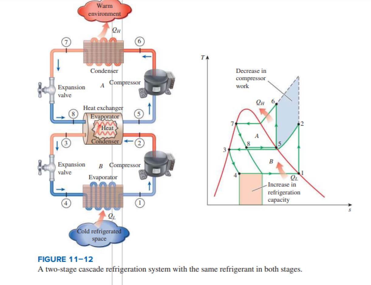
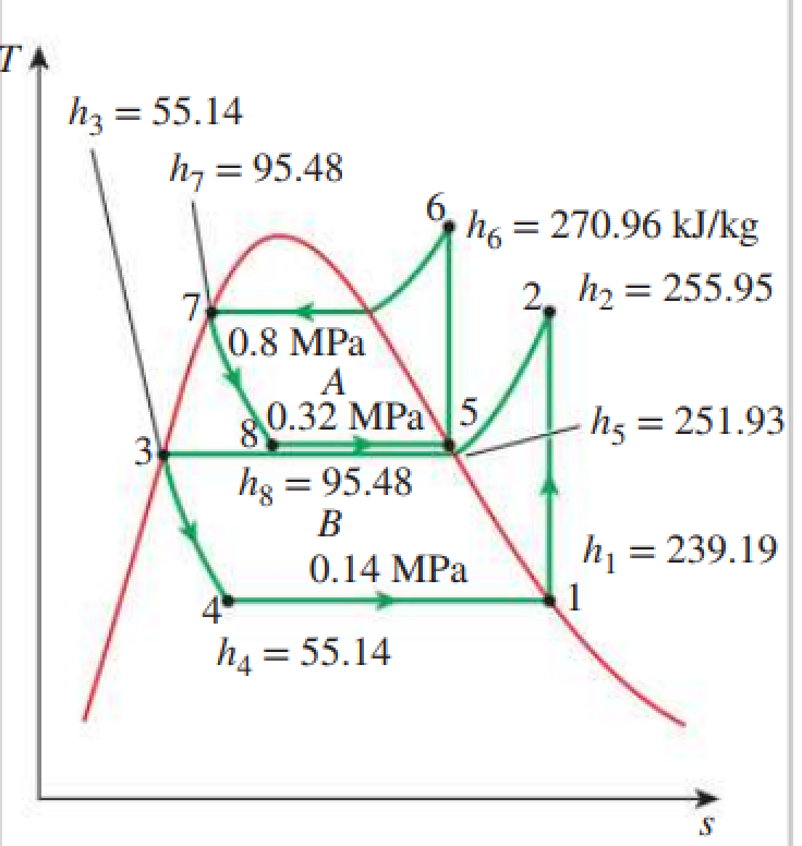
Consider a two-stage cascade refrigeration system operating between the pressure limits of 0.8 and 0.14 MPa.Each stage operates on an ideal vapor-compression refrigeration cycle with refrigerant-134a as the working fluid. Heat rejection from the lower cycle to the upper cycle takes place in an adiabatic counterflow heat exchanger where both streams enter at about 0.32 MPa. (In practice, the working fluid of the lower cycle is at a higher pressure and temperature in the heat exchanger for effective heat transfer.) If the mass flow rate of the refrigerant through the upper cycle is 0.05 kg/s, we determine (a) the mass flow rate of the refrigerant through the lower cycle, (b) the rate of heat removal from the refrigerated space and the power input to the compressor, and (c) the coefficient of performance of this cascade refrigerator.
In[]:=
cycle 1 = UPPER cycle with R134
saturation properties - pressure increment = 0.05 MPaTemperature (C) Pressure (MPa) Enthalpy (kJ/kg) Entropy (J/g*K) Enthalpy (kJ/kg) Entropy (J/g*K)
datasat=;
In[]:=
tblhl=Table[{datasat[[i]][[2]],datasat[[i]][[3]]},{i,1,Length[datasat]}];tblsl=Table[{datasat[[i]][[2]],datasat[[i]][[4]]},{i,1,Length[datasat]}];
In[]:=
fhl=Interpolation[tblhl,InterpolationOrder1];fsl=Interpolation[tblsl,InterpolationOrder1];
In[]:=
tblhv=Table[{datasat[[i]][[2]],datasat[[i]][[5]]},{i,1,Length[datasat]}];tblsv=Table[{datasat[[i]][[2]],datasat[[i]][[6]]},{i,1,Length[datasat]}];
In[]:=
fhv=Interpolation[tblhv,InterpolationOrder1];fsv=Interpolation[tblsv,InterpolationOrder1];
In[]:=
tbltp=Table[{datasat[[i]][[1]],datasat[[i]][[2]]},{i,1,Length[datasat]}];
In[]:=
ftp=Interpolation[tbltp,InterpolationOrder1];
In[]:=
FindRoot[ftp[x]==0.8,{x,1}]
Out[]=
{x31.3275}
In[]:=
FindRoot[ftp[x]==0.32,{x,1}]
Out[]=
{x2.41497}
In[]:=
FindRoot[ftp[x]==0.14,{x,1}]
Out[]=
{x-18.9838}
isobaric properties - pressure = 0.8 MPa
Temperature (C) Pressure (MPa) Enthalpy (kJ/kg) Entropy (J/g*K) Phase
Temperature (C) Pressure (MPa) Enthalpy (kJ/kg) Entropy (J/g*K) Phase
dataisobaric=;
In[]:=
pos=Position[dataisobaric,31.328]
Out[]=
{{284,1},{285,1}}
In[]:=
tblhsv=Table[{dataisobaric[[i]][[1]],dataisobaric[[i]][[3]]},{i,285,Length[dataisobaric]}];tblssv=Table[{dataisobaric[[i]][[1]],dataisobaric[[i]][[4]]},{i,285,Length[dataisobaric]}];tblshsv=Table[{dataisobaric[[i]][[4]],dataisobaric[[i]][[3]]},{i,285,Length[dataisobaric]}];
In[]:=
fshsv=Interpolation[tblshsv];
In[]:=
tblhl1=Table[{datasat[[i]][[3]],datasat[[i]][[2]]},{i,1,Length[datasat]}];tblsl1=Table[{datasat[[i]][[4]],datasat[[i]][[1]]},{i,1,Length[datasat]}];
In[]:=
tblhv1=Table[{datasat[[i]][[5]],datasat[[i]][[2]]},{i,1,Length[datasat]}];tblsv1=Table[{datasat[[i]][[6]],datasat[[i]][[1]]},{i,1,Length[datasat]}];
In[]:=
fhsv=Interpolation[tblhsv,InterpolationOrder1];
In[]:=
fssv=Interpolation[tblssv,InterpolationOrder1];
isobaric properties - pressure = 0.32 MPa
Temperature (C) Pressure (MPa) Enthalpy (kJ/kg) Entropy (J/g*K) Phase
Temperature (C) Pressure (MPa) Enthalpy (kJ/kg) Entropy (J/g*K) Phase
dataisobaric2=;
In[]:=
pos=Position[dataisobaric2,2.4768]
Out[]=
{{224,1},{225,1}}
In[]:=
tblhsv=Table[{dataisobaric2[[i]][[1]],dataisobaric2[[i]][[3]]},{i,225,Length[dataisobaric]}];tblssv=Table[{dataisobaric2[[i]][[1]],dataisobaric2[[i]][[4]]},{i,225,Length[dataisobaric]}];tblshsv=Table[{dataisobaric2[[i]][[4]],dataisobaric2[[i]][[3]]},{i,225,Length[dataisobaric]}];
In[]:=
fshsv2=Interpolation[tblshsv];
In[]:=
tblhl1=Table[{datasat[[i]][[3]],datasat[[i]][[2]]},{i,1,Length[datasat]}];tblsl1=Table[{datasat[[i]][[4]],datasat[[i]][[1]]},{i,1,Length[datasat]}];
In[]:=
tblhv1=Table[{datasat[[i]][[5]],datasat[[i]][[2]]},{i,1,Length[datasat]}];tblsv1=Table[{datasat[[i]][[6]],datasat[[i]][[1]]},{i,1,Length[datasat]}];
In[]:=
fhsv2=Interpolation[tblhsv];
In[]:=
fssv2=Interpolation[tblssv];
In[]:=
Clear[T1,T2,T3,T4,P1,P2,P3,P4,H1,H2,H3,H4,S1,S2,S3,S4,quality]
First, let us determine the unknown variables for points {1, 2, 3, 4} of the Table below:
In[]:=
Grid[{{"point","T °C","P MPa","h kJ/kg","s kJ/kg*K","state"},{2,T2,P2,H2,S2,"sat. vap."},{3,T3,P3,H3,S3,"super heated vap."},{4,T4,P4,H4,S4,"sat. liq."},{1,T1,P1,H1,S1,quality}},Background{None,{Lighter[Yellow,.5],{White,Lighter[Blend[{Blue,Green}],.6]}}},Frame->All,ItemStyle12,Spacings{1.5,1.5}]
Out[]=
point | T °C | P MPa | h kJ/kg | s kJ/kg*K | state |
2 | T2 | P2 | H2 | S2 | sat. vap. |
3 | T3 | P3 | H3 | S3 | super heated vap. |
4 | T4 | P4 | H4 | S4 | sat. liq. |
1 | T1 | P1 | H1 | S1 | quality |
In[]:=
H4=fhl[0.8]
Out[]=
95.5006
In[]:=
S4=fsl[0.8]
Out[]=
0.354137
In[]:=
H2=fhv[0.32]
Out[]=
251.854
In[]:=
S2=fsv[0.32]
Out[]=
0.930194
In[]:=
H1=H4
Out[]=
95.5006
hlsat@P1<H1<hvsat@P1 --- Point 1 is in the two-phase region
In[]:=
H1
Out[]=
95.5006
In[]:=
P1=P2
Out[]=
P2
In[]:=
P2=0.32
Out[]=
0.32
In[]:=
P4=P3
Out[]=
P3
cycle 2 - LOWER cycle with R134A
First, let us determine the unknown variables for points {1, 2, 3, 4} of the Table below:
hlsat@P1<H1<hvsat@P1 --- Point 1 is in the two-phase region
References
References
[1] Çengel, Yunus A., Boles, Michael A., Kanoğlu, Mehmet, Thermodynamics: An Engineering Approach, Ninth Edition, NY: McGraw-Hill, 2019.
CITE THIS NOTEBOOK
CITE THIS NOTEBOOK
A two-stage cascade refrigeration cycle with R134A
by Housam Binous and Ahmed Bellagi
Wolfram Community, STAFF PICKS, February 26, 2025
https://community.wolfram.com/groups/-/m/t/3400487
by Housam Binous and Ahmed Bellagi
Wolfram Community, STAFF PICKS, February 26, 2025
https://community.wolfram.com/groups/-/m/t/3400487