There has been a paper on dark vs bright state of light: https://journals.aps.org/prl/abstract/10.1103/PhysRevLett.134.133603
which provides a new insight into the double-slit experiment and wave-particle duality of light, in quantum theory. Here you can find its implementation in Wolfram Mathematica: https://community.wolfram.com/groups/-/m/t/3461741
I had a correspondence with Celso Jorge Villas-Boas, the first author, and discussing some aspects of their paper. He kindly shared his insight into classical counterpart of dark/bright states of light as a system of coupled oscillator, which he uses in his classes. I explored his idea a bit and I believe it is indeed an excellent classical example, providing some insight into the dark.bright states of light. In this notebook, I provide some codes exploring Celso’s suggestion.
Consider two identical pendulums of length ℓ and mass m, coupled by a torsional spring of stiffness κ at their pivots. Impose the rigid-rod constraints. Then the non‑linear pendulum + torsion-spring ODEs read as:


For small‑angle displacements, the linearizing torques gives:

which can be solved analytically:
In[]:=
ClearAll[ω0,,θ1,θ2,θ10,θ20,v10,v20];$Assumptions={ω0>0,>0};results=FullSimplify@DSolveValue[{D[θ1[t],{t,2}]+θ1[t]+(θ1[t]-θ2[t])==0,D[θ2[t],{t,2}]+θ2[t]-(θ1[t]-θ2[t])==0,θ1[0]==θ10,θ2[0]==θ20,θ1'[0]==v10,θ2'[0]==v20},{θ1[t],θ2[t]},t]
2
ω0
2
ω0
Out[]=
(θ10+θ20)Cos[tω0]+(θ10-θ20)Cost+,(θ10+θ20)Cos[tω0]+(-θ10+θ20)Cost+
1
2
2+
+2
ω0
(v10+v20)Sin[tω0]
ω0
(v10-v20)Sint
2+
2
ω0
2+
2
ω0
1
2
2+
+2
ω0
(v10+v20)Sin[tω0]
ω0
(-v10+v20)Sint
2+
2
ω0
2+
2
ω0
Introduce symmetric and antisymmetric coordinates
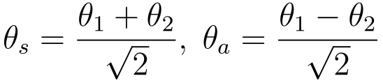
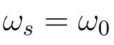
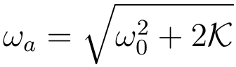
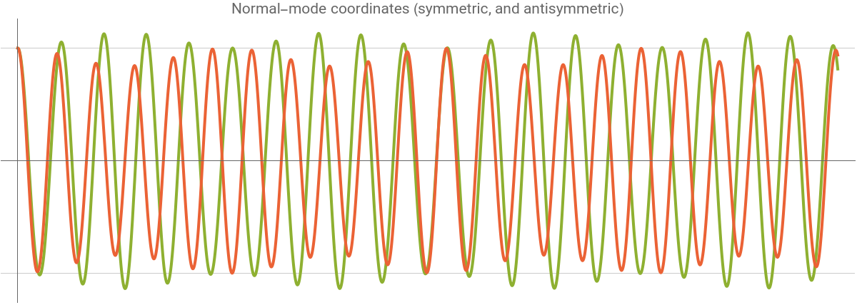
One finds the decoupled ODEs for the two normal‑modes whose frequencies are (which is both pendulums in phase, frequency) and (which is out of phase, frequency)
In[]:=
Subtract@@results//FullSimplifyPlus@@results//FullSimplify
Out[]=
(θ10-θ20)Cost
2+
+2
ω0
(v10-v20)Sint
2+
2
ω0
2+
2
ω0
Out[]=
(θ10+θ20)Cos[tω0]+
(v10+v20)Sin[tω0]
ω0
Solve ODEs for and for different parameters:
θ
1
θ
2
In[]:=
ClearAll[{θ1,θ2,ω0,k,θ10,θ20,v10,v20,tf}]pnd=ParametricNDSolveValue[{D[θ1[t],{t,2}]+Sin[θ1[t]]+(θ1[t]-θ2[t])==0,D[θ2[t],{t,2}]+Sin[θ2[t]]-(θ1[t]-θ2[t])==0,θ1[0]==θ10,θ2[0]==θ20,θ1'[0]==v10,θ2'[0]==v20},{θ1[t],θ2[t]},{t,0,tf},{ω0,,θ10,θ20,v10,v20,tf}]
2
ω0
2
ω0
Out[]=
ParametricFunction


Single‑pendulum displacement
Single‑pendulum displacement
Solve the ODEs for the case of

In[]:=
{th1,th2}=pnd[w0=.3,k=.1,th10=1,th20=0,0,0,tf=20×2πw0];
2
w0
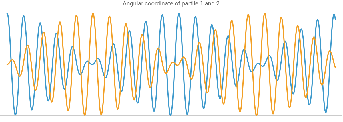
Plot angular coordinates in time:
In[]:=
Plot[Evaluate[{th1,th2}],{t,0,tf},Ticks->None,AspectRatio->1/3,PlotLegends->Placed[{"",""},Right],GridLines->{None,{Max[th10,th20],-Max[th10,th20]}},PlotLabel->"Angular coordinate of partile 1 and 2",ImageSize->600]
θ
1
θ
2
Out[]=


Plot the normal-modes, symmetric and antisymmetric, in time:
In[]:=
PlotEvaluate,,{t,0,tf},Ticks->None,AspectRatio->13,PlotStyle->{ColorData[97][3],ColorData[97][4]},PlotLegends->Placed[{"",""},Right],GridLines->None,{Max[th10+th20,th10-th20],-Max[th10+th20,th10-th20]}
th1+th2
2
th1-th2
2
θ
s
θ
a
2
,PlotLabel->"Normal-mode coordinates (symmetric, and antisymmetric)",ImageSize->600Out[]=


Provide some visualization for angular coordinates:
In[]:=
img1SPD=Plot[Evaluate[{th1,th2}],{t,0,tf},Ticks->None,AspectRatio->1/3,PlotLegends->{"",""}];imgsSPD=TableColumnStyle"Single‑pendulum displacement",Bold,Graphics[{{Line[{{0,0},{2.2,0}}]},{{Gray,Dashed,Circle[{0,0},1,{-π,0}]},{Line[{{0,0},{Sin[th1],-Cos[th1]}}]},{Opacity[.3],FaceForm[ColorData[97][1]],Disk[{0,0},1,{-π/2,-π/2+th1}]},{ColorData[97][1],PointSize[Large],Point[{Sin[th1],-Cos[th1]}]}},Translate[{{Gray,Dashed,Circle[{0,0},1,{-π,0}]},{Line[{{0,0},{Sin[th2],-Cos[th2]}}]},{Opacity[.3],FaceForm[ColorData[97][2]],Disk[{0,0},1,{-π/2,-π/2+th2}]},{ColorData[97][2],PointSize[Large],Point[{Sin[th2],-Cos[th2]}]}},{2.2,0}]},ImageSize->600],Show[img1SPD,Graphics[{{ColorData[97][1],PointSize[.02],Point[{t,th1}]},{ColorData[97][2],PointSize[.02],Point[{t,th2}]}}],ImageSize->600],{t,0,tf,tf/100};
θ
1
θ
2
In[]:=
ExportNotebookDirectory[]<>"Single‑pendulum-displacement.GIF",imgsSPD
Out[]=
Calculate the instantaneous mechanical energy in each bob and plot that versus time:
In[]:=
e1=2+(1-Cos[th1]);e2=2+(1-Cos[th2]);
2
D[th1,t]
2
w0
2
D[th2,t]
2
w0
Plot normalized energies in time:
In[]:=
Plot,,th1,th2,{t,0,tf},Ticks->None,AspectRatio->13,ImageSize->600,PlotStyle->{Automatic,Automatic,Directive[Dashed,Thin,Black],Directive[Thin,Black]},PlotLegends->{"","","",""},PlotLabel->"energy transfer between bobs"
e1
e1+e2
e2
e1+e2
E
1
E
2
θ
1
θ
2
Calculate total energy including the coupling-spring energy
Show total energy is constant in time (up to a numerical error):
Pure symmetric‑mode displacement
Pure symmetric‑mode displacement
Plot angular coordinates in time:
Plot the normal-modes, symmetric and antisymmetric, in time:
Provide some visualization for angular coordinates:
Calculate the instantaneous mechanical energy in each bob and plot that versus time:
Plot normalized energies in time:
Calculate total energy including the coupling-spring energy
Show total energy is constant in time (up to a numerical error):
Pure antisymmetric‑mode displacement
Pure antisymmetric‑mode displacement
Plot angular coordinates in time:
Plot the normal-modes, symmetric and antisymmetric, in time:
Provide some visualization for angular coordinates:
Calculate the instantaneous mechanical energy in each bob and plot that versus time:
Plot normalized energies in time:
Calculate total energy including the coupling-spring energy
Show total energy is constant in time (up to a numerical error):
Adding dissipation
Adding dissipation
We now add viscous damping (e.g. from air resistance or hinge friction) that exerts a torque proportional to each bob’s angular velocity.
The new dissipation term continually removes energy from each bob, so both the in‑phase (bright) and out‑of‑phase (dark) oscillations will decay in amplitude.
Plot angular coordinates in time:
Plot the normal-modes, symmetric and antisymmetric, in time:
Provide some visualization for angular coordinates:
Calculate the instantaneous mechanical energy in each bob and plot that versus time:
Plot normalized energies in time:
Calculate total energy including the coupling-spring energy
Show total energy is constant in time (up to a numerical error):
CITE THIS NOTEBOOK
CITE THIS NOTEBOOK
Wave-particle duality: classical example for dark vs bright states of photons
by Mohammad Bahrami
Wolfram Community, STAFF PICKS, May 20, 2025
https://community.wolfram.com/groups/-/m/t/3464768
by Mohammad Bahrami
Wolfram Community, STAFF PICKS, May 20, 2025
https://community.wolfram.com/groups/-/m/t/3464768