ABSTRACT (original article): We extend the notion of topologically protected semi-metallic band crossings to hyperbolic lattices in a negatively curved plane. Because of their distinct translation group structure, such lattices are associated with a high-dimensional reciprocal space. In addition, they support non-Abelian Bloch states which, unlike conventional Bloch states, acquire a matrix-valued Bloch factor under lattice translations. Combining diverse numerical and analytical approaches, we uncover an unconventional scaling in the density of states at low energies, and illuminate a nodal manifold of codimension five in the reciprocal space. The nodal manifold is topologically protected by a nonzero second Chern number, reminiscent of the characterization of Weyl nodes by the first Chern number. CITATION (original article): Tarun Tummuru, Anffany Chen, Patrick M. Lenggenhager, Titus Neupert, Joseph Maciejko, and Tomáš Bzdušek (2024), Phys. Rev. Lett. 132, 206601. https://doi.org/10.1103/PhysRevLett.132.206601
Initialization
Initialization
Dirac model on the {8,8} lattice
Dirac model on the {8,8} lattice
Import cells
Import cells
We first import the cell, model, and supercell model graphs as produced by the HyperCells package (see https://github.com/patrick-lenggenhager/HyperCells for the package repository):
In[]:=
pcell=ImportCellGraphString[Import[FileNameJoin[{"data","cells","(2,8,8)_T2.6_3.hcc"}]]];
pcmodel=ImportModelGraphString[Import[FileNameJoin[{"data","cells","{8,8}-tess_T2.6_3.hcm"}]]];
We consider the following sequence of supercells, defined in terms of quotients given in https://www.math.auckland.ac.nz/~conder/TriangleGroupQuotients101.txt by M. Conder:
In[]:=
supercells={"T3.11","T5.13","T9.20","T17.29","T33.44"};
In[]:=
scmodels=Association[#->ImportSupercellModelGraphString[Import[FileNameJoin[{"data","cells",ToString@StringForm["{8,8}-tess_T2.6_3_sc-``.hcs",#]}]]]&/@supercells];
Model on the primitive cell T2.6
Model on the primitive cell T2.6
We define the model on the primitive cell given by the quotient group T2.6. The primitive cell (Wigner-Seitz unit cell) forms an octagon with a single site at its center and nearest neighbors in adjacent copies of the cell:
In[]:=
VisualizeModelGraph[pcmodel,Elements<|ShowCellGraphFlattened{},ShowCellBoundary{ShowEdgeIdentificationTrue}|>,CellGraphpcell,NumberOfGenerations2,ImageSize300]
Out[]=
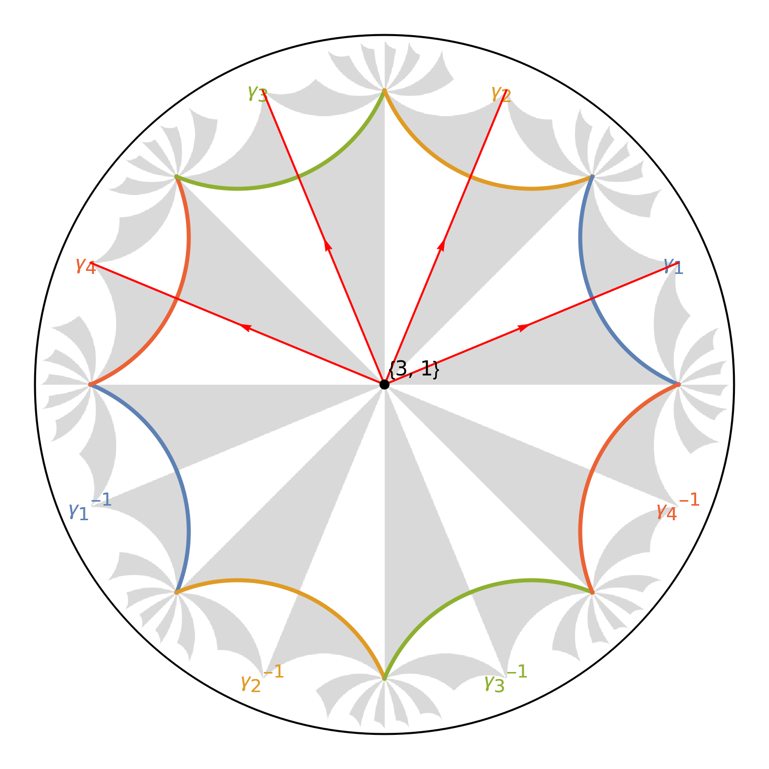
The model consists of four orbitals placed at that site and coupled to its nearest neighbors with Gamma matrices depending on the four distinct directions
γ
1
In[]:=
σ0=PauliMatrix[0];σx=PauliMatrix[1];σy=PauliMatrix[2];σz=PauliMatrix[3];[1]=KroneckerProduct[σx,σ0];[2]=KroneckerProduct[σy,σ0];[3]=KroneckerProduct[σz,σx];[4]=KroneckerProduct[σz,σy];[5]=KroneckerProduct[σz,σz];
In[]:=
hopping=AssociationThread[EdgeList@pcmodel["Graph"]->(([5]+[ToExpression@StringReplace[#,RegularExpression["g(\\d)"]:>"$1"]])/2&/@pcmodel["EdgeTranslations"])]
Out[]=
{3,1}{3,1},0,,0,0,-,0,,,0,-,0,0,,0,,{3,1}{3,1},,0,0,-,-,0,0,0,0,-,-,0,0,,,{3,1}{3,1},0,,0,0,-,0,,-,0,-,0,0,-,0,,{3,1}{3,1},,0,0,,-,0,0,0,0,-,-,0,0,-,
{1,{1,1,5}}
1
2
2
1
2
2
2
1
2
2
1
2
{1,{2,4,8}}
1
2
1
2
1
2
1
2
1
2
1
2
1
2
1
2
{1,{3,2,6}}
1
2
1
2
1
2
1
2
1
2
1
2
1
2
1
2
{1,{4,3,7}}
1
2
2
2
1
2
1
2
2
2
1
2
Additionally, there is an onsite Dirac mass :
m
In[]:=
onsite[m_]:={{m,0,0,0},{0,-m,0,0},{0,0,-m,0},{0,0,0,m}}&
With this information, we construct the Abelian Bloch Hamiltonian on the primitive cell:
In[]:=
(Hpc=FullSimplify[AbelianBlochHamiltonian[pcmodel,4&,onsite[m],hopping][[2]]])//MatrixForm
Out[]//MatrixForm=
m+Cos[k1]+Cos[k2]+Cos[k3]+Cos[k4] | -Sin[k3]+Sin[k4] | -Sin[k1]+Sin[k2] | 0 |
-Sin[k3]-Sin[k4] | -m-Cos[k1]-Cos[k2]-Cos[k3]-Cos[k4] | 0 | -Sin[k1]+Sin[k2] |
-Sin[k1]-Sin[k2] | 0 | -m-Cos[k1]-Cos[k2]-Cos[k3]-Cos[k4] | Sin[k3]-Sin[k4] |
0 | -Sin[k1]-Sin[k2] | Sin[k3]+Sin[k4] | m+Cos[k1]+Cos[k2]+Cos[k3]+Cos[k4] |
We export the matrix
Export[FileNameJoin[{"data","ABH","ABH_{8,8}-dirac_T2.6.dat"}],Hpc,"Table"];
Density of states
Density of states
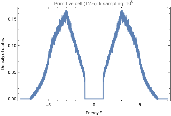
We approximate the density of states by randomly sampling momenta, i.e., one-dimensional irreducible representations, and diagonalizing the Bloch Hamiltonian evaluated at those. For faster evaluation, we compile the expression for the Bloch Hamiltonian for the specific Dirac mass of interest, here :
m=3
In[]:=
Hpccf=AbelianBlochHamiltonian[pcmodel,4&,onsite[3],hopping,CompileFunction->True]
Out[]=
CompiledFunction


The computation of the density of states (DOS) can take advantage of the independence of different momentum sectors and can therefore be parallelized:
In[]:=
ComputeDOS[cfH_,Npts_,Nruns_,{Emin_,Emax_},dE_]:=Module[{data,tot,dimk=Length[cfH[[2]]]},data=Transpose[{MovingAverage[Range[Emin,Emax,dE],2],Total@ParallelTable[HistogramList[Flatten@Table[Chop@Eigenvalues[cfH@@RandomReal[{-Pi,Pi},dimk]],{i,1,Round[Npts/Nruns]}],{Emin,Emax,dE}][[2]],{j,1,Nruns},Method"FinestGrained"]}];tot=Total@data[[;;,2]];{#1,#2/dE/tot}&@@@data]
As stated in the paper, we compute the DOS with an energy resolution of 0.005 (but for demonstration purposes with a smaller sampling of instead of )
6
10
9
10
In[]:=
dospc=ComputeDOS[Hpccf,10^6,32,{-8-0.005,8},0.005];
In[]:=
ListLinePlotdospc,FrameTrue,FrameStyleBlack,FrameLabel{"Energy E","Density of states"},PlotRangeAll,PlotLabel->"Primitive cell (T2.6); k sampling: "
6
10
Out[]=
The full data with larger sampling is stored as data/DOS/dos_{8,8}-dirac_T2.6_{3}.dat and we can import and plot it:
In[]:=
ListLinePlotImport[FileNameJoin[{"data","DOS","dos_{8,8}-dirac_T2.6_{3}.dat"}]],FrameTrue,FrameStyleBlack,FrameLabel{"Energy E","Density of states"},PlotRangeAll,PlotLabel->"Primitive cell (T2.6); k sampling: "
9
10
Out[]=
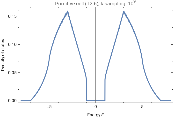
We observe an energy gap, i.e., a region of energy with no states, around .
E=0
Model on the supercells
Model on the supercells
The model is extended to the supercells in the sequence by translation symmetry, which allows us to construct the Abelian Bloch Hamiltonians on the supercells
2-Supercell
2-Supercell
Of particular interest is the 2-supercell Bloch Hamiltonian, which we have used to compute a low-energy expansion and find the nodal manifold:
See the full matrix in full size here: https://www.wolframcloud.com/obj/2dcf11f5-0f18-4308-84af-c805fd725d6f
Density of states
Density of states
Increasingly better approximations of the true density of states in the thermodynamic limit are obtained by considering one-dimensional irreducible representations on increasingly larger supercells. This is the supercell method, P. M. Lenggenhager et al (2023). Phys. Rev. Lett. 131, 226401. https://doi.org/10.1103/PhysRevLett.131.226401. Wolfram Community post and code: https://community.wolfram.com/groups/-/m/t/3131734
Again, we first compile the expressions for the Abelian Bloch Hamiltonians to speed up the evaluation:
Again, we first compile the expressions for the Abelian Bloch Hamiltonians to speed up the evaluation:
We plot the successively better approximations of the (normalized) density of states as obtained from successively larger supercells:
The full data is stored as data/DOS/dos_{8,8}-dirac_<quot>_{<m>}.dat, where <quot> is the corresponding quotient and <m> the value of the Dirac mass. We import and plot it due to the reduced noise:
CITE THIS NOTEBOOK
CITE THIS NOTEBOOK
Hyperbolic non-Abelian semimetal
by Tarun Tummuru, Anffany Chen, Patrick M. Lenggenhager, Titus Neupert, Joseph Maciejko, and Tomáš Bzdušek
Wolfram Community, STAFF PICKS, May 21, 2024
https://community.wolfram.com/groups/-/m/t/3180067
by Tarun Tummuru, Anffany Chen, Patrick M. Lenggenhager, Titus Neupert, Joseph Maciejko, and Tomáš Bzdušek
Wolfram Community, STAFF PICKS, May 21, 2024
https://community.wolfram.com/groups/-/m/t/3180067