The intrinsic geometry of one-dimensional Riemannian manifolds does not distinguish a circle from an ellipse with uniform length discretization. When graphs are discretized using uniformly spaced vertices with respect to arc length, intrinsic distance statistics between pairs of vertices are therefore identical for the two curves. In contrast, extrinsic observables depend on the embedding. In particular, when Euclidean chord lengths between pairs of vertices are considered, the resulting distributions differ. The goal of this project is to investigate whether analogous signatures arise for the two-dimensional case by comparing a sphere with an ellipsoid under a (non) uniform-length discretization. Unlike the one-dimensional case, a generic ellipsoid is intrinsically distinct from a sphere, suggesting that intrinsic graph observables may already encode information about its geometry.
Introduction
Introduction
A central problem in discrete geometry is to determine which geometric properties of a continuous space can be recovered from a finite graph that approximates it. Familiar quantities from Riemannian geometry—such as dimension, curvature, and geodesic distance—can be studied in this setting. In this spirit, the broader infrageometry program may be viewed as an exploratory framework for investigating whether large graphs admit effective geometric descriptions at sufficiently large scales.
This essay considers the distribution of distances between pairs of vertices as a possible geometric observable. Our motivating question is whether such distributions can provide information about isotropy or anisotropy. This is treated as a question to be investigated, not as an assumption: distance distributions may depend on the chosen discretization and do not, in general, determine a geometry uniquely.
We first compare a circle and an ellipse. When both are discretized uniformly with respect to arc length, their intrinsic distance distributions agree, while their Euclidean chord-distance distributions reflect their different embeddings. We then study the analogous two-dimensional comparison between a sphere and an ellipsoid. Since a generic ellipsoid is intrinsically different from a sphere, we ask whether distributions of approximate geodesic distances can detect aspects of this difference, including anisotropy.
Benchmarking on Discretization
Benchmarking on Discretization
To benchmark our experiment we consider approximations of Riemannian manifolds by graphs. We start with manifolds embedded as subsets in . Any discretization method is good to preserve geometry if we keep edge lengths between vertices by remembering the coordinates of vertices (as VertexCoordinates) and the lengths of edges (as EdgeWeight). To obtain such a graph, we have to identify vertices with a point cloud approximating the manifold and decide which vertices we connect by edges. However, If we want to forget edge lengths and just have bare graphs from which we would like to extract the geometry, we have to take the uniform length discretization, which, by definition, approximate well the Euclidean surface distance.
n
R
◼
So, to benchmark our experiment (observing how the histogram relates to the a,b,c), we can:
◼
Take the default discretization with edgelengths,
◼
Or the uniform length discretization (as bare graph).
Distribution of mutual distances
Distribution of mutual distances
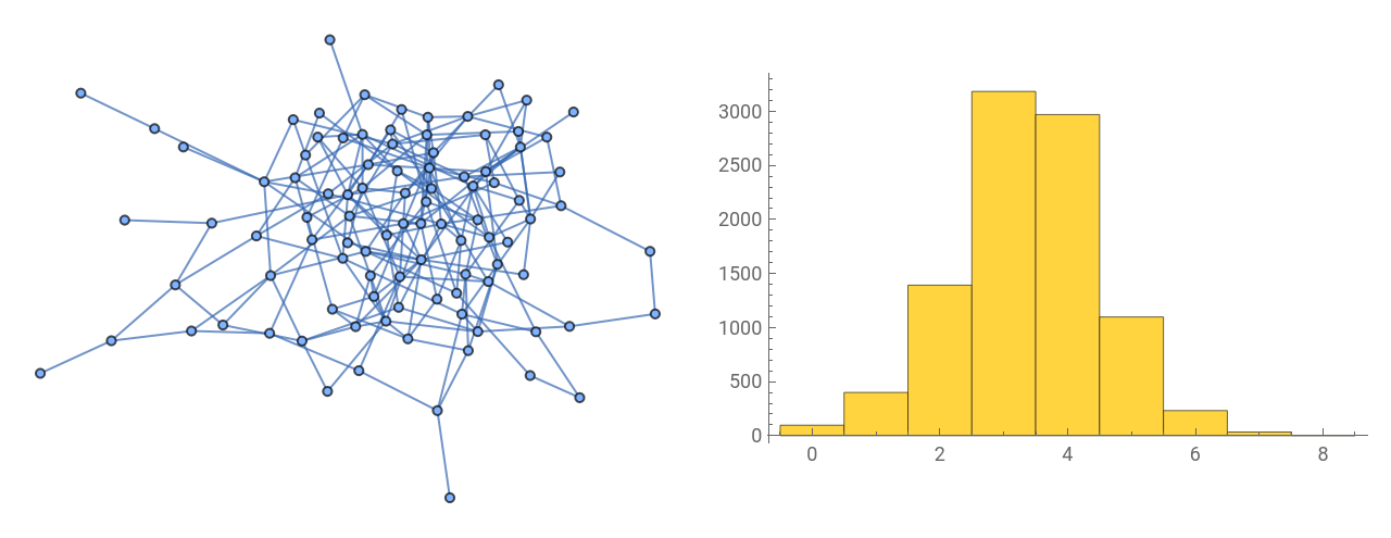
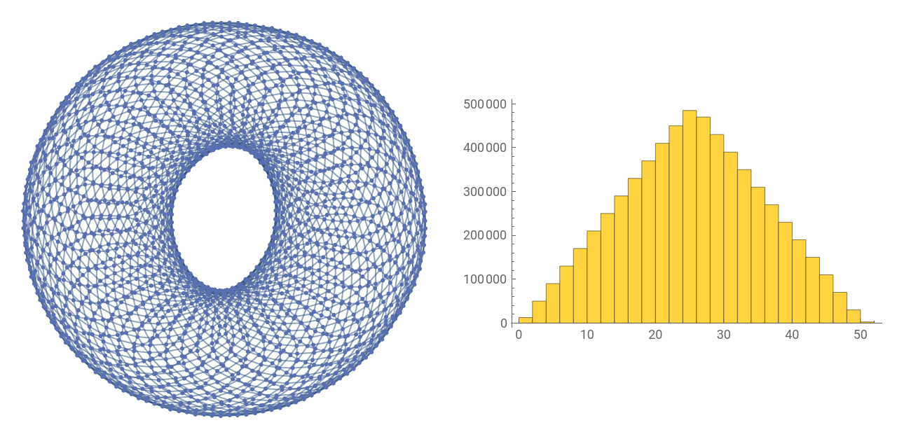
Given a random graph we can compute the distribution of mutual shortest path distances. Here we don’t consider any edge weights, so the function GraphDistanceMatrix consider the length of any edge to be 1.
In[]:=
ClearAll["Global`*"];GraphicsRow[{g=With[{graph=RandomGraph[{100,200}]},Subgraph[graph,First@WeaklyConnectedComponents[graph]]],Histogram@Flatten@GraphDistanceMatrix[g]}]
Out[]=
In[]:=
ClearAll["Global`*"];GraphicsRow[{g=TorusGraph[{50,50}],Histogram@Flatten@GraphDistanceMatrix[g]}]
Out[]=
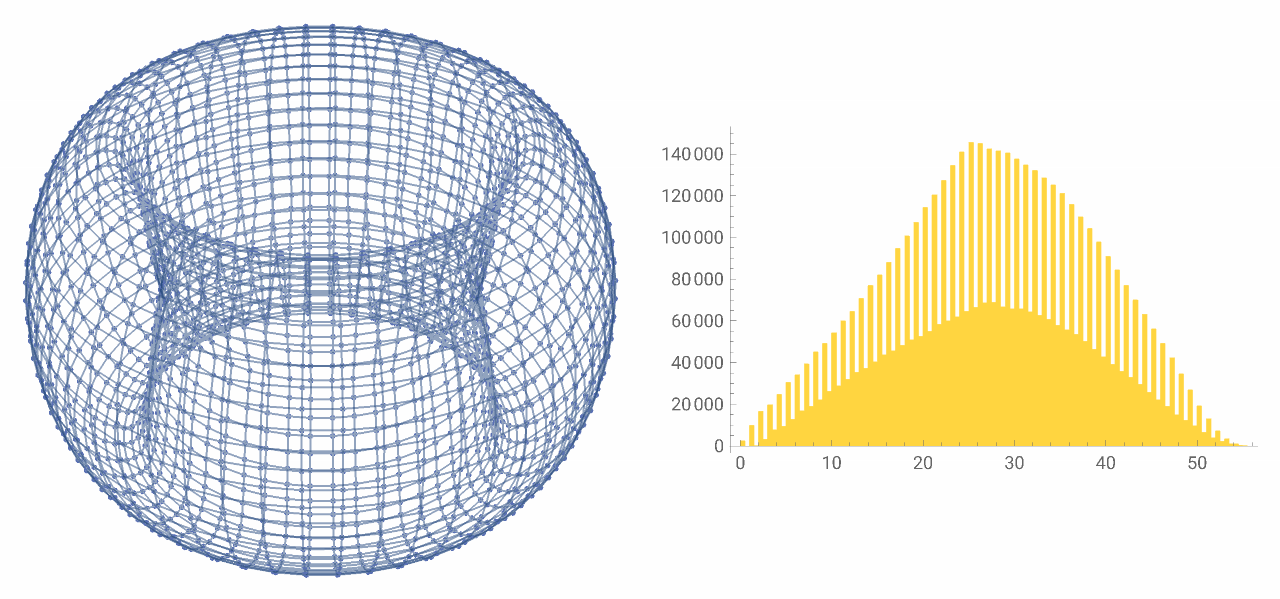
However, we can also do the same experiment with different edge weights, and then the histogram, of course, changes. Note: The GraphDistanceMatrix function in this case actually takes into account the edge weights.
Out[]=
Uniform Length Discretization for the Circle vs Ellipse
Uniform Length Discretization for the Circle vs Ellipse
Circle (arc length on the circle and Euclidean chord distance)
Circle (arc length on the circle and Euclidean chord distance)
For a circle, constructing a uniform-length discretization is straightforward. Since the circle has constant curvature and symmetry, we can place vertices at equal angular intervals; these intervals correspond to equal arc lengths along the curve. In other words, dividing the full angle of the circle evenly produces vertices that are uniformly spaced with respect to the intrinsic length, or arc length. The resulting arc length histogram therefore looks like this:
Out[]=
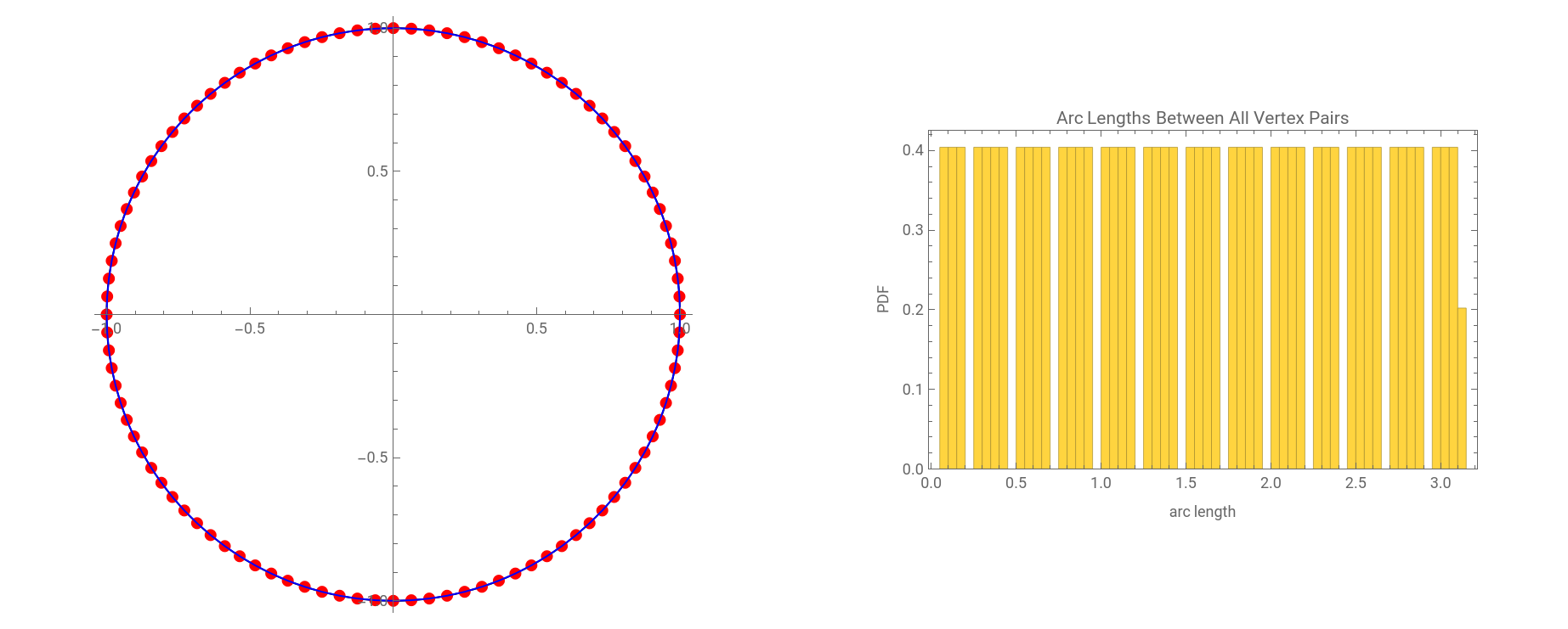
For 100 uniformly spaced vertices on the circle, every step separation from 1 to 49 occurs exactly 100 times. For example, there are 100 pairs of vertices that are one step apart, 100 pairs that are two steps apart, and so on. Since the vertices are uniformly distributed, these step separations correspond to equally spaced arc lengths around the circle.
The only exception occurs at a separation of 50 steps, where the two vertices are diametrically opposite. Each opposite pair is counted only once, so this distance occurs 50 times instead of 100. This is why the final bar in the arc length histogram is lower than the others.
The only exception occurs at a separation of 50 steps, where the two vertices are diametrically opposite. Each opposite pair is counted only once, so this distance occurs 50 times instead of 100. This is why the final bar in the arc length histogram is lower than the others.
For the extrinsic distance, however, the histogram of Euclidean chord lengths between all pairs of vertices has a more interesting shape.
Out[]=
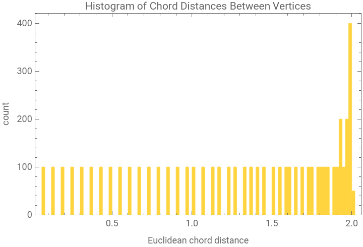
If two points are chosen uniformly on the unit circle, or equivalently if we consider all pairs of uniformly spaced vertices, the chord length is d , where θ is the angular separation between the points. Since θ is uniformly distributed on [0,π], its density is P(θ) = . Changing variables from θ to d we use P(θ) dθ = P(d)dd which gives P(d) = . This density diverges as d approaches 2, the maximum chord length on the unit circle. In the histogram, this appears as a buildup near the endpoint. The divergence is an integrable square-root singularity: the total area under the curve remains finite, even though the density itself becomes arbitrarily large near the maximum chord distance.
=2Sin(θ/2)
1
π
1
π√(1-(d/2)^2)
Ellipse (arc length on the ellipse and Euclidean chord distance)
Ellipse (arc length on the ellipse and Euclidean chord distance)
For the ellipse, unlike the circle, an equal angular spacing does not imply equal arc length spacing. We can compare three different discretization strategies:
1
. Uniform Angle: the angle between neighboring vertices is constant.
∠(,)
x
i
x
i+1
2
.Uniform Arc length: the arc length dl between neighboring vertices is constant.
x
i+1
∫
x
i
3
.Uniform Chord Distance: the chord distance + between neighboring vertices is constant
2
(-)
x
i
x
i+1
2
(-)
y
i
y
i+1
Out[]=

Out[]=

From the intrinsic point of view, where distance is measured by arc length along the curve, the ellipse does not produce a distribution that is fundamentally different from the circle. Uniform arc length spacing only records separation along the one-dimensional curve. See the middle histogram in comparison to the one associated with the circle (both have uniform Arc length between two neighboring vertices). This is expected since the only thing that distinguishes the circle from the ellipse as Riemannian manifold is the embedding. The extrinsic geometry, however, tells a different story.
Out[]=

When the vertices are chosen so that neighboring chord lengths are equal, the distribution of Euclidean chord distances between all pairs of vertices becomes skewed and asymmetric, reflecting the varying curvature of the ellipse. Compare the right histogram with the one associated with the circle!
When vertices are placed at equal arc length intervals, the resulting intrinsic distance structure is essentially uniform in both cases. The difference appears when we look extrinsically, using Euclidean chord distances in the ambient plane. For the circle, equal angular spacing, equal arc length spacing, and equal neighboring chord spacing all align because of the circle’s symmetry. For the ellipse, these notions separate: equal angular spacing no longer gives equal arc lengths, and equal arc length spacing does not imply equal chord lengths between neighboring vertices. Thus the ellipse reveals how curvature and embedding affect the extrinsic distribution of distances, even when the intrinsic discretization appears uniform.
To see that the embedding is the main tool for distinguishing an ellipse from a circle, use the same code above but inquire forgetting coordinates as in: VertexCoordinates->{}. In that case, there is no way to distinguish between a circle and an ellipse. intrinsically, they are the same!
To see that the embedding is the main tool for distinguishing an ellipse from a circle, use the same code above but inquire forgetting coordinates as in: VertexCoordinates->{}. In that case, there is no way to distinguish between a circle and an ellipse. intrinsically, they are the same!
Weighted and Unweighted Graph
Weighted and Unweighted Graph
We have an example here where we forget the vertex coordinates and thus forgetting the embedding. We are still preserving the Edge lengths as Edge weights. The result of preserving edge lengths is preserving the internal geometry even though the extrinsic geometry looks different. See the first and the second graph below. Compare the following properties of a graph
Each edge has a label and weight. Every vertex has a label and a “coordinate” assigned by the algorithm. One can think of it as a special label. The default embedding algorithm by Mathematica is the spring electric embedding.
Sphere vs Ellipsoid
Sphere vs Ellipsoid
Sphere (intrinsic and chord distances)
Sphere (intrinsic and chord distances)
We begin by considering how far we can go in discretizing the sphere with exactly equal edge lengths. The following code uses the 12 vertices of an icosahedron to discretize the sphere. In this case, the 30 neighboring edges all have the same Euclidean length with the requirement that every vertex share the same number of faces.
If we require a regular triangular discretization of the sphere, meaning that every face is an equilateral triangle and every neighboring Euclidean edge length is exactly equal, then the largest possible example is the icosahedron, with 12 vertices. The only regular triangular cases are the tetrahedron with 4 vertices, the octahedron with 6 vertices, and the icosahedron with 12 vertices. Thus, the icosahedron is the finest exact regular triangular discretization of the sphere.
If we allow other Platonic solids whose faces are not necessarily triangles, then the largest number of vertices is 20, achieved by the dodecahedron. Its neighboring edges are also all equal, but its faces are pentagons rather than triangles. For larger values, such as n=100 or n=1000, we can construct good approximately uniform meshes of the sphere, as shown below, but we should not expect all neighboring Euclidean edge lengths to be exactly equal.
After the exact icosahedral case, we move to a larger discretization of the sphere. In this case, the mesh is no longer perfectly uniform: the neighboring Euclidean edge lengths are close to one another, but they are not all exactly equal. This is visible in the edge-length histogram, where the lengths are concentrated in a narrow range rather than collapsing to a single value. Thus, for larger meshes, the edge lengths remain within a relatively narrow range, but they are not uniformly distributed and do not define an exact equal-edge discretization.
Ellipsoid (intrinsic and chord distances)
Ellipsoid (intrinsic and chord distances)
In this section we perform a nonuniform discretization to address our question. In the second plot, the Euclidean chord distance between neighboring vertices are not the same. With that in mind, can we notice any difference with the sphere at the level of intrinsic geometry? In other words, can we compute the arc length instead of Euclidean chord distances and get any indication of anisotropy between the ellipsoid and the sphere?
For the ellipse boundary, there is only one curve, so arc length between vertices is easy to compute. For an ellipsoid surface, however, there are infinitely many surface paths between two vertices. Usually we want the shortest path along the surface, called the geodesic distance. For a discretized ellipsoid mesh, the simple approximation is to use shortest paths along the mesh edges. On the last plot, we compute the Euclidean chord distance between arbitrary pairs of vertices on the mesh. The plots below are for a triaxial ellipsoid with a>b>c.
For the ellipse boundary, there is only one curve, so arc length between vertices is easy to compute. For an ellipsoid surface, however, there are infinitely many surface paths between two vertices. Usually we want the shortest path along the surface, called the geodesic distance. For a discretized ellipsoid mesh, the simple approximation is to use shortest paths along the mesh edges. On the last plot, we compute the Euclidean chord distance between arbitrary pairs of vertices on the mesh. The plots below are for a triaxial ellipsoid with a>b>c.
And for an oblate spheroid, that is an ellipsoid with a=b>c, we have
And for a prolate spheroid, that is an ellipsoid with a>b=c, we have
Is there a way to get approximate uniform length?
Is there a way to get approximate uniform length?
Sprinkling vs Uniform length vs triangulated Mesh
Sprinkling vs Uniform length vs triangulated Mesh
Why exact uniform length could be difficult to impose?
Why exact uniform length could be difficult to impose?
Requiring equal Euclidean distances between neighboring vertices on a sphere or ellipsoid is generically an over-constrained condition. Suppose we have a closed triangular mesh with V vertices on a fixed ellipsoid. Each vertex has two degrees of freedom, corresponding to its position on the surface, and we also introduce one additional unknown: the common edge length. Thus the total number of unknowns is 2V+1.
Now consider the number of edge-length constraints. If the mesh is triangular, then each face has three edges, but each edge is shared by two faces, so the face by face edge count gives 3F = 2E. For a sphere-like closed surface, Euler’s formula gives V-E+F=2. Combining these two relations gives E = 3V - 6. Since each edge imposes one constraint, namely that its Euclidean length equals the common edge length, the difference between the degrees of freedom and the constraints is 2 V + 1 - (3 V - 6) = 7 - V. Therefore, once V > 7, the system has more constraints than unknowns. This means that, generically, we should not expect to be able to place vertices on a sphere or ellipsoid so that every neighboring pair has exactly the same Euclidean chord length. For a rigorous proof, one would have to consider the rank of the Jacobian of the system of constraints.
This is only a counting argument, not a rigorous impossibility proof for every special case. Highly symmetric configurations may still exist. However, it explains why exact uniform edge-length discretizations are difficult to impose in general on a full closed triangular mesh.
Concluding Remarks and Future Directions
Concluding Remarks and Future Directions
The goal of this project was to investigate whether aspects of the geometry represented by a graph can be inferred from the distribution of pairwise vertex distances. We benchmarked this experiment using three discretization strategies for an ellipsoid. Among the examples considered, the approximately uniform-edge-length discretization most closely reproduced the expected geometric behavior after the edge lengths and embedding information were removed. We also examined how the mean, variance, and skewness of the distance distribution vary with the parameters of the ellipsoid. A natural next step is to quantify these relationships and determine which statistical moments provide the most reliable signatures of anisotropy.
The attempt to construct uniform-edge-length discretizations also raised theoretical questions. A simple counting argument suggests that exact equal-edge-length triangulations are generally overconstrained, although special symmetric configurations may exist. It would therefore be interesting to study the existence of discretizations satisfying prescribed properties, including triangulations with equal or approximately equal edge lengths and trivalent dual graphs. Using a nonuniform-edge-length mesh in the two-dimensional case, we found that a sphere and an ellipsoid can be distinguished through their intrinsic distance distributions. Future work should repeat this comparison using the approximate uniform-edge-length method developed above.
A broader motivation for this work comes from the Kasner solution in general relativity, which provides a simple anisotropic model for spacetime behavior near certain singular regimes. The question of whether graphs or hypergraphs could represent aspects of Kasner-like anisotropy was suggested by Elena Caceres in a discussion following her presentation, “Large N Models, Holography, Black Holes & Hypergraphs” Establishing such a connection would be a long-term goal, particularly because the discretization of Lorentzian manifolds presents additional conceptual difficulties. The present work takes a preliminary step by asking how anisotropy, and more generally geometric information, may be detected using observables defined directly on graphs.
Acknowledgments
Acknowledgments
I would like to thank my mentors, Pavel Hajek and Carlos Zapata-Carratala. I am grateful to Pavel for proposing this project, for our fruitful discussions throughout the summer program, and for his extensive help with the computational implementation. I thank Carlos for his talks on the hypergraph rewriting model and for his insights into the algebraic framework underlying the broader research program. I also thank Elena Caceres for her presentation at the Wolfram Conference in Austin, and for a series of stimulating discussions that motivated the question of whether Kasner-like anisotropy might be represented using graphs or hypergraphs. Finally, I thank Stephen Wolfram for his support of the program and all the staff members for creating such an engaging and enjoyable experience.
References
References
◼
Caceres, Elena. “Large N Models, Holography, Black Holes & Hypergraphs.” Presentation at Bridging Wolfram Models and Mathematical Physics, Austin, Texas, 2026. https://wolframinstitute.org/wolfram-models-conference
AI Disclosure
AI Disclosure
The following generative AI tools were used in this project: [Codex, version 26.707.62119 ]. They were used for brainstorming, literature review, debugging code and editing prose. All code and written content were reviewed, understood and approved by the author.
CITE THIS NOTEBOOK
CITE THIS NOTEBOOK
Anisotropy of Space From Discretization
by Merna Youssef
Wolfram Community, STAFF PICKS, July 16, 2026
https://community.wolfram.com/groups/-/m/t/3762711
by Merna Youssef
Wolfram Community, STAFF PICKS, July 16, 2026
https://community.wolfram.com/groups/-/m/t/3762711