The study of nonlinear dynamical systems in lattices is an area of research with continuously growing interest.The first systematic studies of these systems emerged in the late 1930 s,thanks to the work of Frenkel and Kontorova on crystal dislocations.These studies led to the formulation of the discrete Klein-Gordon equation (DKG).Specifically,in 1939,Frenkel and Kontorova proposed a model that describes the structure and dynamics of a crystal lattice in a dislocation core.The FK model has become one of the fundamental models in physics,as it has been proven to reliably describe significant phenomena observed in discrete media.The equation we will examine is a variation of the following form:
̈
θ
n
θ
n+1
θ
n
θ
n-1
2
ω
a
n
The process described involves approximating a nonlinear differential equation through the Taylor method and simplifying it into a linear model.Let’s analyze step by step the process from the initial equation to its final form.For small angles,sin θ can be approximated through the Taylor series as:
sinθ≈θ-
3
θ
3!
We substitute F(θ) in the original equation with the Taylor approximation:
̈
θ
n
θ
n+1
θ
n
θ
n-1
2
ω
θ
n
3
θ
n
3!
To map this equation to a linear model,we consider the angles Subscript[θ, n] to correspond to displacements Subscript[x, n] in a mass-spring system.Thus,the equation transforms into:
2
d
x
n
d
2
t
x
n+1
x
n
x
n-1
2
ω
x
n
3
x
n
3!
The exact value of β depends on the mapping of coefficients in the Taylor approximation and its application to the specific physical problem. Our main goal is to derive results regarding stability and convergence in nonlinear lattices under nonlinear conditions.We will examine the basic characteristics of the discrete Klein-Gordon equation:
-κ(-2+)-β
2
d
x
n
d
2
t
x
n+1
x
n
x
n-1
2
ω
d
x
n
3
x
n
The term represents a generalization of Hooke’s law in a discrete and nonlinear context,where is the elasticity constant that indicates a body’s resistance to deformation,reflecting the interaction of a point with its two immediate neighboring points in a discrete structure.The difference -2+ provides a measure of curvature or the difference in the slope of the function at point . The term reveals how the motion of the body evolves.In the second term of the equation,the term -β describes a nonlinear dynamic affecting the n-th particle,with representing the square of a frequency that determines the intensity of the system’s linear response to the particles’ displacements from their equilibrium,while the term introduces a nonlinearity in the equation,with being a constant that determines the intensity of the nonlinear interaction,taking into account the nonlinear forces acting on the particle,which become significant as the displacements from equilibrium increase.
κ(-2+)
x
n+1
x
n
x
n-1
κ
x
n+1
x
n
x
n-1
n
2
d
x
n
d
2
t
2
ω
d
x
n
3
x
n
2
ω
d
-β
3
x
n
β
This model is often used to describe the opening of the DNA double helix during processes such as transcription.The model focuses on the transverse motion of the base pairs,which can be represented by a set of coupled nonlinear differential equations.
In[]:=
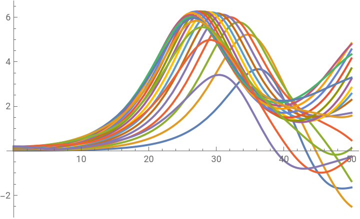
(*AdjustedParameters*)numBases=20;(*Numberofbasepairs*)kappa=0.1;(*Elasticityconstant*)omegaD=0.2;(*Frequencyterm*)beta=0.05;(*Nonlinearitycoefficient*)(*Initialpositionsandvelocitiesforeachbasepair*)initialPositions=Table[x[n][0]==0.01n,{n,1,numBases}];initialVelocities=Table[x[n]'[0]==0,{n,1,numBases}];(*Assuminginitialreststate*)(*BoundaryConditions*)boundaryConditions={x[0][t]==0,x[numBases+1][t]==0};(*Equations*)equations=Table[x[n]''[t]-kappa(x[n+1][t]-2x[n][t]+x[n-1][t])==omegaD^2(x[n][t]-betax[n][t]^3),{n,1,numBases}];(*SolveNumerically*)solution=NDSolveValue[{equations,initialPositions,initialVelocities,boundaryConditions},Table[x[n],{n,1,numBases}],{t,0,50}];(*Visualization*)Plot[Evaluate[Table[solution[[n]][t],{n,1,numBases}]],{t,0,50},PlotLegends->Table[StringJoin["Base ",ToString[n]],{n,1,numBases}],PlotRange->All]
Out[]=


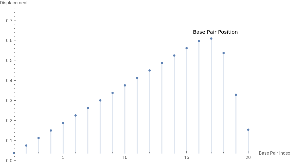
Displacements at t==10
In[]:=
(*Chooseaspecifictimeforthesnapshot*)snapshotTime=10;(*GenerateDiscretePlotfortheDNAmodelatthesnapshottime*)DiscretePlot[solution[[n]][snapshotTime],{n,1,numBases},PlotRange->All,PlotStyle->PointSize[Medium],PlotLabels->Placed["Base Pair Position",Above],AxesLabel->{"Base Pair Index","Displacement"}]

Out[]=
In[]:=
(*Generatedatafor3Dplot*)data=Flatten[Table[{n,t,solution[[n]][t]},{n,1,numBases},{t,0,50,0.5}],1];(*3DPlot*)ListPointPlot3D[data,AxesLabel->{"Base Pair","Time","Displacement"},PlotRange->All,ColorFunction->"Rainbow",PlotStyle->PointSize[Small]]
Out[]=

In[]:=
(*Choosespecifictimepointsforvisualization*)timePoints={0,10,20,30,40,50};(*Generatedataforeachtimepoint*)dataAtTimePoints=Table[Table[{n,time,solution[[n]][time]},{n,1,numBases}],{time,timePoints}];(*3DDiscretePlot*)Graphics3D[{Table[{Hue[time/Max[timePoints]],PointSize[0.02],Point[data]},{time,timePoints},{data,dataAtTimePoints[[Position[timePoints,time][[1,1]]]]}]},Axes->True,AxesLabel->{"Base Pair","Time","Displacement"},BoxRatios->{1,1,0.5},PlotRange->All]
Out[]=

CITE THIS NOTEBOOK
CITE THIS NOTEBOOK
GenoDynamics: Exploring DNA Oscillations with the Discrete Klein-Gordon Framework
by Athanasios Paraskevopoulos
Wolfram Community, STAFF PICKS, February 25, 2024
https://community.wolfram.com/groups/-/m/t/3129486
by Athanasios Paraskevopoulos
Wolfram Community, STAFF PICKS, February 25, 2024
https://community.wolfram.com/groups/-/m/t/3129486