Of Christmas lights: the nine colourings of the Holt graph
by Jeremy Tan / Parcly Taxel
National University of Singapore
by Jeremy Tan / Parcly Taxel
National University of Singapore
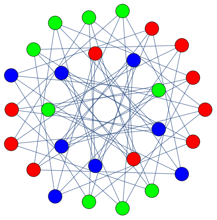
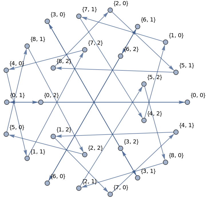
The non-degenerate unit-distance embedding of the Holt graph shown above is one of several such embeddings from my Shibuya repository I submitted to Eric Weisstein around October and November 2021 which ended up in Mathematica 13. Most embeddings are either of cubic symmetric graphs or braced polygons, so I was genuinely surprised when my GAP-powered search program turned this up – it is indeed the unique embedding with the highest possible symmetry of ( in GAP).
The graph is 3-colourable, and when I first discovered it I made a symmetric 3-colouring of it by hand. That left a lingering question of how many inequivalent colourings it had, however; two colourings are considered equivalent if there is a combination of graph automorphism and colour permutation (to be referred as combined symmetry) that turns one into the other. As a kind of Christmas present I made for myself, I have went ahead and shown that there are exactly nine inequivalent colourings.
D
9
D
18
The graph is 3-colourable, and when I first discovered it I made a symmetric 3-colouring of it by hand. That left a lingering question of how many inequivalent colourings it had, however; two colourings are considered equivalent if there is a combination of graph automorphism and colour permutation (to be referred as combined symmetry) that turns one into the other. As a kind of Christmas present I made for myself, I have went ahead and shown that there are exactly nine inequivalent colourings.
My exact construction of the unit-distance embedding’s vertex coordinates, together with a description of the edges simpler than that given at MathWorld, is below. Every one of the 54 graph automorphisms preserves the shown directions of all edges, hence the half-transitive property.
radius[i_]:=With[{t=4Cos[2^iPi/9]^2},{1,-1,-1}[[i+1]]Sqrt[Root[#^3+(1-t)#^2+t#-t/3&,1]]];vinds=Flatten[Table[{i,j},{i,0,8},{j,0,2}],1];vcoords=ReIm[Flatten[Table[radius[j]Exp[2iIPi/9],{i,0,8},{j,0,2}]]];edges=Flatten[Table[{i,j}{Mod[i+2^(j+1)s,9],Mod[j+1,3]},{i,0,8},{j,0,2},{s,{1,-1}}],3];Graph[vinds,DirectedEdge@@@edges,VertexCoordinatesThread[vinds->vcoords],VertexLabelsAutomatic]
Out[]=
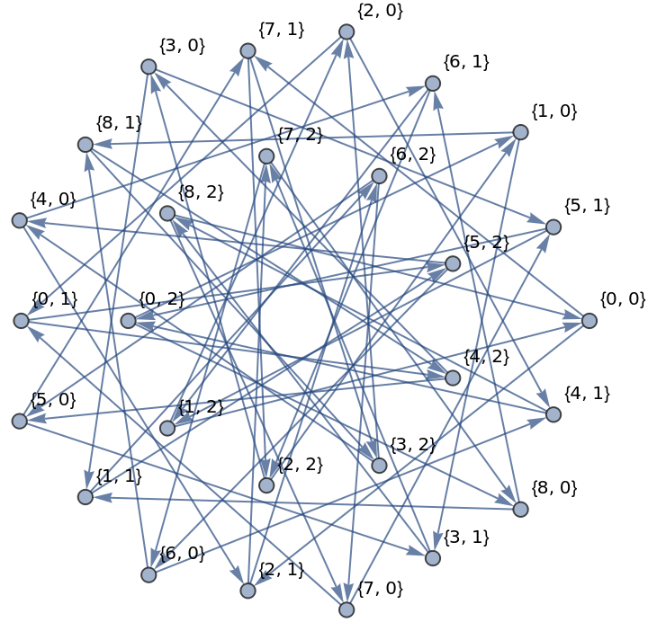
The automorphism group has these three generators, the first two of which are generators for the symmetry group of the embedding. The third generator then looks vaguely like a snowflake, but I was not expecting that appearance.
D
9
In[]:=
o9=Cycles[{{1,4,7,10,13,16,19,22,25},{2,5,8,11,14,17,20,23,26},{3,6,9,12,15,18,21,24,27}}];o2=Cycles[{{4,25},{5,26},{6,27},{7,22},{8,23},{9,24},{10,19},{11,20},{12,21},{13,16},{14,17},{15,18}}];o3=Cycles[{{1,2,3},{4,23,15},{5,24,13},{6,22,14},{7,17,27},{8,18,25},{9,16,26},{10,11,12},{19,20,21}}];{e9,e2,e3}=Map[(QuotientRemainder[#-1,3]&),Thread[Range[27]PermutationList[#]],{-1}]&/@{o9,o2,o3};
Graph[vinds,e9,VertexCoordinatesThread[vinds->vcoords],VertexLabelsAutomatic]
Out[]=
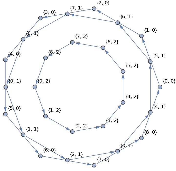
Graph[vinds,e2,VertexCoordinatesThread[vinds->vcoords],VertexLabelsAutomatic]
Out[]=
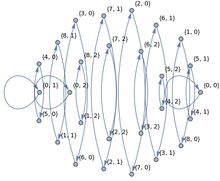
Graph[vinds,e3,VertexCoordinatesThread[vinds->vcoords],VertexLabelsAutomatic]
Out[]=
The actual task of finding the inequivalent colourings was not done in Mathematica. It took a Python script interfacing with a dedicated SAT solver (I used CaDiCaL) to generate all 948 colourings, as predicted by the chromatic polynomial. A GAP program then determined the orbits of the action of the combined symmetry group (=324 elements) on the colourings. Both programs can be found here.
Nine orbits appeared, with the following representatives:
54·3!
Nine orbits appeared, with the following representatives:
In[]:=
ineqs={{0,0,0,1,0,2,1,2,0,2,2,2,0,2,1,0,1,2,1,1,1,2,1,0,2,0,1},{0,0,0,1,1,1,2,2,2,0,0,0,1,1,1,2,2,2,0,0,0,1,1,1,2,2,2},{0,0,0,1,1,2,1,2,2,0,0,0,1,2,1,2,1,2,0,0,0,2,1,1,2,2,1},{0,0,1,0,0,1,2,1,2,1,1,0,2,0,2,0,0,1,2,0,2,1,1,0,2,1,2},{0,0,1,0,0,1,2,1,2,1,1,0,2,0,2,0,2,1,2,0,2,1,1,0,2,1,2},{0,0,1,0,0,1,2,2,1,2,2,0,1,0,1,0,0,2,1,0,1,2,2,0,2,2,1},{0,0,1,0,0,2,1,1,2,1,1,0,2,0,2,0,0,1,2,0,2,1,1,0,2,1,2},{0,0,1,2,0,1,2,1,1,2,1,1,2,0,1,0,0,1,2,0,2,1,2,0,2,0,2},{0,1,2,0,1,2,0,1,2,0,1,2,0,1,2,0,1,2,0,1,2,0,1,2,0,1,2}}/.{0->RGBColor[1,0,0],1->RGBColor[0,1,0],2->RGBColor[0,0,1]};
Most of their symmetries (or lack thereof) only become apparent upon colouring the embeddings. In LRTB order and pre-dividing by 6 for the colours, the colourings below have 3, 1, 9, 27, 27, 27, 54, 9, 1 equivalents under graph automorphism.
G=Graph[vinds,edges,VertexCoordinatesThread[vinds->vcoords],VertexSizeLarge];GraphicsGrid[ArrayReshape[Annotate[G,VertexStyle->Thread[VertexList[G]->#]]&/@ineqs,{3,3}],ImageSizeFull]
Out[]=
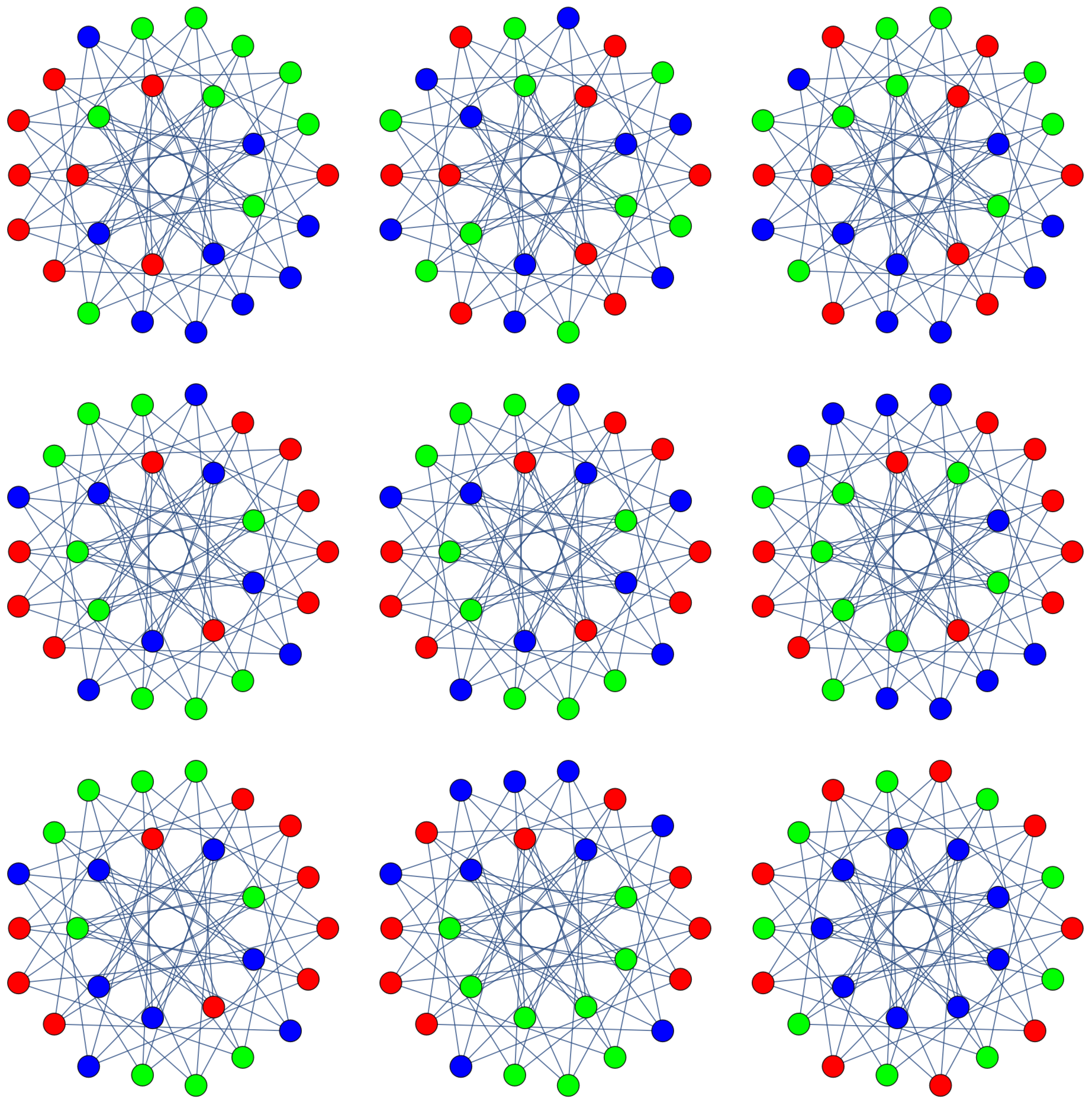
The embedding at the top of this notebook is the “fully asymmetric” 54-equivalent one; every non-trivial combined symmetry yields a different colouring per se. It is almost symmetric though, in that switching the {6, 1} vertex colour between red and yellow has the same effect as a combined symmetry.
Proceeding to more symmetric colourings, the three with 27 equivalents all have a recognisable flip symmetry, as does the second 9-equivalent. The first 9-equivalent has the combined symmetry of a flip automorphism (here across the x-axis) and a blue/green swap, while the 3-equivalent clearly has threefold symmetry in its colour arrangement. All the distinct-per-se equivalents of these last three colourings can, again obviously, be generated by rotating the whole graph.
The first 1-equivalent (i.e. totally invariant under graph automorphism) colouring is the one I found when I discovered the embedding, but the second one was a pleasant surprise.
Happy Hearth’s Warming!