I’m excited to announce that the notebook version of Laplace Transforms in Theory and Practice: A Computational Approach by Hrachya Khachatryan was published by Wolfram Media on March 12, 2026 for all the world to learn this beautiful subject. You can get your copy of the book free here: [https://www.wolfram-media.com/products/laplace-transforms-in-theory-and-practice/].
The Laplace transform provides effective and easy means for solving many problems that arise in mathematics, science and engineering. It is one of the main tools available for solving differential equations. This book presents the theory and applications of the Laplace transform. Early chapters explain the transform, essential properties, methods for evaluation and numerical algorithms. Middle chapters concentrate on the inverse transform, complex inversion, series and asymptotic expansions and even multivariate and numerical inverse Laplace transforms. Later chapters are dedicated to applications of the Laplace transform, from ordinary differential equations to partial, integral and even fractional differential equations. These topics are typically found in university courses on applied mathematics and electrical engineering.
The powerful symbolic and numerical computational capabilities of Wolfram Language, along with its robust visualization tools provide an ideal environment in which to study this subject.
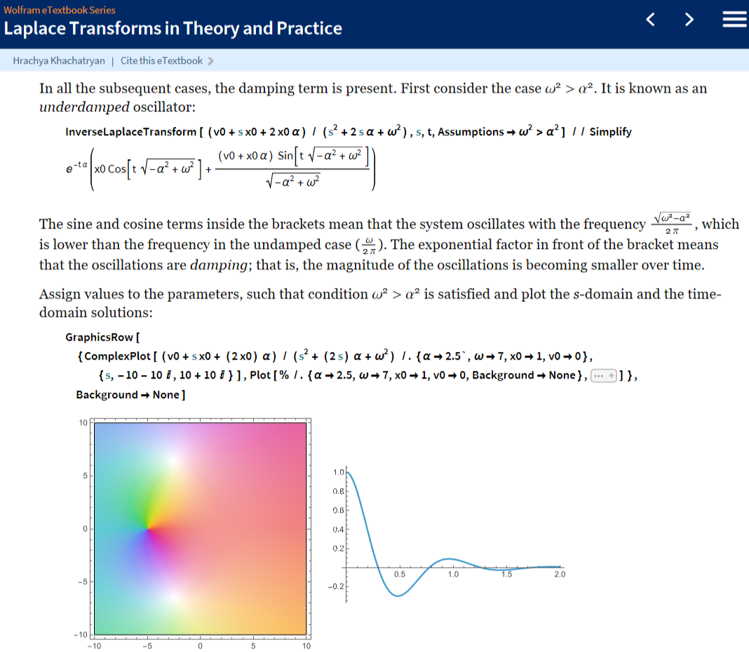
Sophisticated proofs are generally avoided to focus instead on explaining essential concepts in detail. Many examples and exercises are included to help the reader understand and apply the practical side of Laplace transform theory. Solutions to exercises are presented at the end of each chapter and even a summarizing “Laplace Transforms in a Nutshell” chapter is included as a study guide for readers. The book concludes with a sample exam covering most of the chapters and a table of Laplace a inverse Laplace transforms.
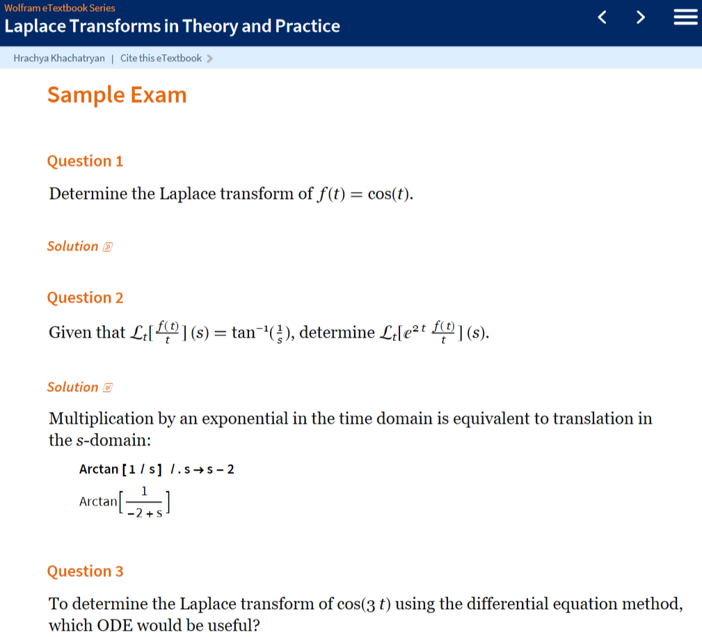
Following the success of Essentials of Complex Analysis: A Computational Approach by Marco Saragnese, this book deepens the Wolfram eTextbook Series in tackling typically abstract and pure mathematics with Wolfram Language tools. Expect more books in this series on advanced topics soon, including Special Functions from Theory to Application: A Computational Approach by Tigran Ishkhanyan in the next few months. Also keep an eye on Wolfram social channels and our series webpage for opportunities to sign up for more prerelease editions of forthcoming books in the series. For more information, please contact publishing@wolfram.com.
Book Introduction
Book Introduction
The Laplace transform is such an effective tool for solving problems in the fields of science and engineering that it deserves a book of its own. It’s one of the main tools available for solving differential equations—both ordinary differential equations (ODEs) and partial differential equations (PDEs). In this book, we will dive deep into the theory behind the Laplace transform, but we’ll also leave plenty of room to study practical applications. To simplify explanations and visualizations, we will use Wolfram Language—a powerful, knowledge-based language designed to be a comprehensive tool for computation and programming across many domains, from mathematics and science to engineering and data analysis. It’s powerful function, together with and , makes it an ideal software companion for this course.
This book focuses exclusively on the Laplace transform and its inverse in both everyday words and mathematical terms. We avoid presenting sophisticated proofs and focus instead on explaining essential concepts in detail. A large number of examples and exercises are included to help the reader digest the material and to highlight the practical side of Laplace transform theory. Readers will also be presented with solutions to the exercises at the end of the each chapter.
The 25 chapters presented here are organized into three sections. The first and second sections introduce the Laplace transform and its inverse respectively, covering essential properties such as linearity, scaling, translation theorems and the convolution theorem. We also explain methods for evaluating Laplace and inverse Laplace transforms, including the Bromwich inversion formula for the inverse transform, asymptotic expansion methods, numerical methods and more. The third section is dedicated to applications of the Laplace transform in differential equations (e.g. ODEs, PDEs, integral equations, fractional differential equations) across various fields of physics and engineering. Engineers will find this section useful for studying control systems.
A wide range of readers will benefit from this material. Primarily, it is designed to be used by undergraduates as a textbook for a formal course on Laplace transforms or as supplementary material for such a course. The book also contains more advanced material (e.g. chapters on asymptotic expansions of the Laplace transform and numerical inverse Laplace transforms), which can be beneficial for both graduate students and researchers. We have tried to keep the book self-contained; however, some prior knowledge of calculus and complex analysis is required for a better understanding of the book.
Hrachya Khachatryan,
Wolfram Research, Inc.
Wolfram Research, Inc.
Below is a sample lesson from the book
Sample Chapter: 14 | Complex Inversion
Sample Chapter: 14 | Complex Inversion
In this chapter, the complex inversion formula for the inverse Laplace transform will be discussed. Until now, various techniques (such as table lookup for the Laplace transform, the convolution method, partial fraction decomposition, etc.) have been employed to obtain the inverse of a given -domain function. Although these methods prove useful in many instances—indeed, for most application-oriented examples, applying some of these techniques described in the previous chapters is sufficient—there is still a desire to find a formula for the inversion.
s
In Chapter 1, a formula for the Laplace transform was provided. However, possessing a formula doesn’t guarantee an immediate determination of the final answer. For instance, in the Laplace transform formula, the challenging part was the integration process. Nevertheless, having a formula means that one can represent the inverse (the time-domain function) using that formula. This is the principal difference of the inversion formula from other methods. The methods described so far either lead to a complete answer or they lead nowhere. In conclusion, the motivation for having an inversion formula lies in its generality: it provides concrete operations that one needs to apply on the -domain function to find the inverse. These operations do not depend on the choice of the function.
s
The inverse Fourier transform will be used to obtain a formula for the inverse Laplace transform. Suppose that is the -domain function and suppose that is its time-domain counterpart. Then according to the Laplace transform formula:
F(s)
s
f(t)
F(s)exp(-st)f(t)t
∞
∫
0
This integral converges when the real part of is large enough: . The function is then analytic in that right half-plane. For the region , is defined via analytic continuation.
s
Re(s)>a
F(s)
Re(s)<a
F(s)
First, one needs to increase the domain of the integration to the whole real axis:
F(s)exp(-st)f(t)h(t)t
+∞
∫
-∞
where is the Heaviside function.
h(t)
As a next step, represent as a sum of its real and imaginary parts: :
s
sc+y
F(s)exp(-yt)(exp(-ct)h(t)f(t))t
+∞
∫
-∞
Therefore, can be thought to be the Fourier transform of the function . Since and is the real part of , then .
F(s)
exp(-ct)h(t)f(t)
Re(s)>a
c
s
c>a
One can now employ the inverse Fourier formula to express function in terms of :
exp(-ct)h(t)f(t)
F(s)
exp(-ct)h(t)f(t)(1/(2π))exp(yt)F(s)y
+∞
∫
-∞
Assume and multiply both sides of the equation above by :
t>0
exp(ct)
f(t)(1/(2π))exp((*y+c)t)F(s)y
+∞
∫
-∞
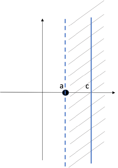
Notice that , since . Notice that when goes from to , then goes from to , along the vertical line in the complex plane:
y=*s
1
*y+cs
y
-∞
+∞
s
c-∞
c+∞
In conclusion, one obtains:
f(t)(1/(2π))exp(t*s)F(s)s
c+∞
∫
c-∞
(
1
)Formula (
1
) is known as the complex inversion formula or the Fourier–Mellin–Bromwich (FMB) integral. The vertical line along which the integration is performed is known as the Bromwich line.One can see the complex inversion formula is very similar to the Laplace transform formula with the exchange of functions and . Also, for the Laplace transform the integration is along the real line; in the FMB formula the integration is along the vertical line in the complex plane instead. This is an important subtlety. It makes the direct evaluation of ( (as long as the vertical line lies in the region , where is analytic). On the right-hand side, the integration is performed from to , and therefore it might be not be obvious why the integration should be independent on the choice of . Suppose that the integration is performed along ≠c (such that >a):
F(s)⟷f(t)
exp(st)⟷exp(-st)
1
) a more challenging task as compared with the integration along the real positive axis in the Laplace transform. Before showing how to tackle the integral in (1
), a few further remarks about the complex inversion formula are in order. First, notice that in (1
) the left-hand side is independent of the choice of c=Re(s)
Re(s)>a
F(s)
c-∞
c+∞
c
′
c
′
c
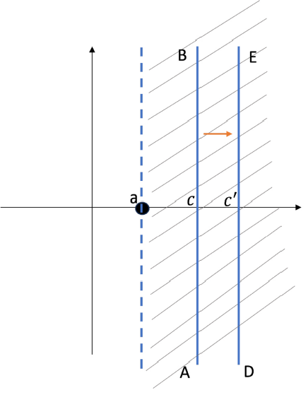
Since both vertical lines are on the left of the dashed line that is in the region where is analytic, then one can use Cauchy’s theorem for the analytic functions. It states that the integral along the closed contour ABED is zero. Assume that function at , therefore the integrals along BE and DA are 0 in the limit as . Therefore, the sum of the integrals along AB and ED is 0, which proves that integration doesn’t depend on choice of .
F(s)
F(s)->0
s->∞
s->∞
c
Next, a few examples will be given that describe different scenarios of singularities and how one needs to properly close the contour to use Cauchy’s residue theorem to evaluate the contour integral.
Consider the following function:
Therefore:
Its poles are:
Consider the following function:
One cannot simply close the contour to the left by adding a semicircle like in the previous examples, because it will cross the branch cut at some point and this will hinder us from applying Cauchy’s residue theorem (remember that in the theorem it is assumed that the function is analytic on the contour). Instead, one can choose the contour as follows:
Evaluating the last integral, one obtains:
Consider the final example, with a logarithmic branch cut discontinuity:
The integral along FG is:
Since the contour ABCDEFGHKM doesn’t contain any singularities inside, then by Cauchy’s theorem the contour integral is 0. This allows us to express the Bromwich integral along the vertical line as a sum of integrals along DE and FG:
Summary
Summary
◼
An inversion formula is presented to find the inverse.
◼
The complex inversion formula, also known as the Fourier–Mellin–Bromwich integral, is obtained by linking the Laplace transform to the Fourier transform and employing the inverse Fourier transform.
◼
The inversion formula is used to invert functions with poles, essential singularities and branch cuts.
Exercises
Exercises
Exercise 1
Exercise 1
Exercise 2
Exercise 2
Exercise 3
Exercise 3
Exercise 4
Exercise 4
Exercise 5
Exercise 5
CITE THIS NOTEBOOK
CITE THIS NOTEBOOK
Laplace Transforms in Theory and Practice: A Computational Approach now available in notebook format
by Hrachya Khachatryan
Wolfram Community, STAFF PICKS, March 18, 2026
https://community.wolfram.com/groups/-/m/t/3665842
by Hrachya Khachatryan
Wolfram Community, STAFF PICKS, March 18, 2026
https://community.wolfram.com/groups/-/m/t/3665842