ORIGINAL ARTICLE: Paixão, M.M.A., Lima, H.S. Numerical validation of Ehrenfest theorem in a Bohmian perspective for non-conservative systems. Eur. Phys. J. Plus 138, 549 (2023). DOI: https://doi.org/10.1140/epjp/s13360-023-04023-z
Article Abstract: In this work we make a high precision numerical study of the Ehrenfest theorem using the Bohmian approach, where we obtain classical solutions from the quantum trajectories performing the Bohmian averages. We analyse the one-dimensional quantum harmonic and Duffing oscillator cases, finding numerical solutions of the time-dependent Schrödinger equation and the guidance equation for different sets of initial conditions and connects these results with the corresponding classical solutions. We also investigate the effect of introducing external forces of three types: a simple constant force, a fast-acting Gaussian impulse, and an oscillatory force with different frequencies. In the last case, the resonance in the quantum trajectories was observed.
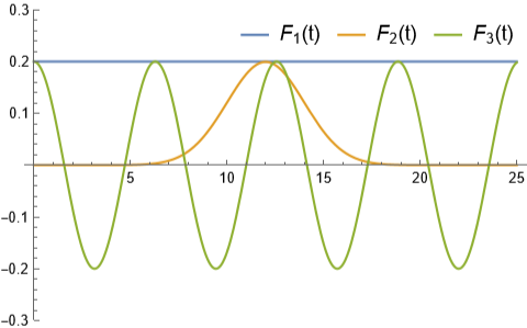
In the framework of Bohmian mechanics [1,2,3], also known as the pilot wave interpretation, the motion of the quantum particles is guided by the wave function Ψ (,t) = R(,t) through the guidance equations =S, (1) where S(,t) is the phase and represents the position. By inserting the polar form of Ψ into the Schrödinger equation Ψ = i ℏ Ψ, with the Hamiltonian , we obtain two real equations ++V+Q=0, (2) +.+S=0. (3) The first one is the Hamilton-Jacobi equation with an additional quantum potential , while the second represents a continuity equation with probability density and a velocity field given by Eq. (1). So, integrating the guidance equation we obtain the trajectories of the quantum particles, which we assume to be initially distributed according to in order to have a probabilistic interpretation. In Bohmian Mechanics, the one-dimensional version of the Ehrenfest theorem is given by [4] , (4) <p=-<, (5) where represents the mean value of a physical property , which can be approximated for a large number of trajectories by the following average:, where N is the total number of trajectories. In this program, based on work [5], we consider the quantum harmonic oscillator case driven by an external force. The associated Hamiltonian is . As examples we consider three distinct forces: 1) A constant force with ; 2) A Gaussian impulse modeled by ; 3) A sinusoidal signal . In addition, we also consider the Duffing oscillator, where a quartic perturbation is introduced to the harmonic potential. The program is structured as follows: Solve the one-dimensional time-dependent Schrödinger equation, taking as initial condition a linear superposition, with the same weight, of the eigenstates of the quantum harmonic oscillator; Solve the guidance equations for a set of initial positions distributed according to ; Export the associated quantum trajectories and compute the Bohmian averages.
x
x
iS(,t)ℏ
x
e
d
x
dt
∇
m
x
x
H
∂
t
H=2m+V(,t)
2
p
x
∂S
∂t
2
S
∇
2m
∂
2
R
∂t
∇
2
R
∇
m
Q=-R
2
ℏ
2m
2
∇
R
2
R
2
Ψ,t=0
x
m<x=<p
d
dt
>
dBB
>
dBB
d
dt
>
dBB
dV
dx
>
dBB
<O
>
dBB
O
<O≈((t))
>
dBB
1
N
N
∑
i=1
O
i
H=+-F(t)x
2
p
2m
1
2
2
mω
0
2
x
F(t)=C,
C∈
F(t)=exp
1
2π
2
σ
-
2
(t-)
t
μ
2
2
σ
F(t)=Acos(ωt)
2
(|Ψ(x,0)|)
Note: This is an open-source code developed by Matheus M. A. Paixão and Henrique S. Lima, both from the Brazilian Center for Research in Physics (CBPF). Feel free to use, reproduce, and modify this code in its entirety or in part of it. We kindly request to justly cite the appropriate Wolfram page together with our work [5].
Initial definitions:
Initial definitions:
In[]:=
Quit;
$HistoryLength=0;Needs["NumericalCalculus`"];Needs["DifferentialEquations`InterpolatingFunctionAnatomy`"];
Parameters
boundary=15;time=50;tμ=12.0;σ=2;A=0.2;anorm=1/(Pi^(1/4.0));α=0.1;Ω=1.0;strx0="n="<>ToString[Nstates];
External Forces
F1[t_]:=A;F2[t_]:=(1/(σ*Sqrt[2*Pi]))*Exp;F3[t_]:=A*Cos[Ω*t];Plot[{F1[t],F2[t],F3[t]},{t,0,time/2},PlotRange{Automatic,{-0.3,0.3}},PlotLegends{Placed[LineLegend[{"(t)","(t)","(t)"},LegendLayout{"Row",1}],{Right,Top}]}]
-
2
(t-tμ)
2*σ^2
F
1
F
2
F
3
Potential
VF[x_,t_]:=*x^2+(*(α/4)*x^4*)-F3[t]*x;
1
2
Eigenfunctions of Quantum Harmonic Oscillator
psi[x_,n_]:=(1/Sqrt[(2^n)*n!])*anorm*E^(-x^2/2)*HermiteH[n,x];
Initial condition for Schrödinger equation
cond[x_,n_]:=(1/Sqrt[n+1])*Sum[psi[x,i],{i,0,n}];Nstates=0;
Out[]=
Solving the Schrödinger equation assuming a Cartesian decomposition: ψ(x,t)= ψr(x,t) + iψi(x,t)
Solving the Schrödinger equation assuming a Cartesian decomposition: (x,t) + i(x,t)
ψ(x,t)=
ψ
r
ψ
i
Progress updates variables
$HistoryLength=0;showStatus[status_]:=LinkWrite[$ParentLink,SetNotebookStatusLine[FrontEnd`EvaluationNotebook[],ToString[status]]];clearStatus[]:=showStatus[""];clearStatus[]
Using the wave function decomposition , the Schrödinger equation can be decomposed into two real equations, given in terms of op1 and op2 defined below
ψ=+
ψ
r
iψ
i
op1=-(1/2)D[Ψr[x,t],{x,2}]+VF[x,t]*Ψr[x,t]+D[Ψi[x,t],t];op2=-(1/2)D[Ψi[x,t],{x,2}]+VF[x,t]*Ψi[x,t]-D[Ψr[x,t],t];
Method
mol[n:_Integer|{_Integer..},o_:"Pseudospectral"]:={"MethodOfLines","SpatialDiscretization"->{"TensorProductGrid","MaxPoints"->n,"MinPoints"->n,"DifferenceOrder"->o}};
Numerical computation of the wave function . The method variables should be changed as we vary the external force, the potential V, and the initial condition
sol=NDSolve[{op10,op20,Ψr[x,0]cond[x,Nstates],Ψi[x,0]0,Ψr[boundary,t]0,Ψr[-boundary,t]0,Ψi[boundary,t]0,Ψi[-boundary,t]0},{Ψr,Ψi},{t,0,time},{x,-boundary,boundary},Method->mol[300,6],(*MaxSteps->∞,*)AccuracyGoal5,PrecisionGoal5,EvaluationMonitor:>showStatus["t = "<>ToString[CForm[t]]]];
dBB interpretation: ψ(x,t) = R(x,t)*i*S(x,t)e
dBB interpretation: ψ(x,t) =
R(x,t)*
i*S(x,t)
e
Polar Form of the wave function:
ψ=
iS
Re
R[x_,t_]:=Sqrt[Ψr[x,t]^2+Ψi[x,t]^2]/.sol;S[x_,t_]:=ArcTan[Ψi[x,t]/Ψr[x,t]]/.sol;
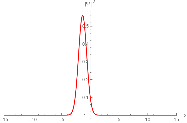
Wave function normalization
testTime=time;PlotEvaluate[R[x,testTime]^2/.sol],{x,-boundary,boundary},PlotRangeAll,(*ColorFunctionColorData["TemperatureMap"]*)PlotStyle{Red},AxesLabel{"x","|Ψ"},PlotPoints1000,MeshFalseNumInt=NIntegrate[R[x,testTime]^2,{x,-boundary,boundary},Method"GaussBerntsenEspelidRule"];"I(|ψ(x,t="<>ToString[testTime]<>")|^2) = "<>ToString[NumInt[[1]]]"Error(t="<>ToString[testTime]<>") = "<>ToString[Abs[1-NumInt[[1]]]]
2
|
Out[]=
Wave function DensityPlot
Velocity field
Solving the guidance equations
Computing the quantum trajectories for this set of initial conditions
Save data trajectories
Export data
End Export data
x (t) versus t plot
Momentum
Export data
End Export data
Quantum trajectories in phase space
Bohmian Averages
Bohmian Averages
Mean values of x and p over the quantum trajectories
Solution of the analogue classic system
x versus t
x versus t
Plot of the analogue classic solution
Plot of the Bohmian Averages
Combined Plot
Classic phase space
Plot of the Bohmian Averages
Combined Plot
References
References
[1] L. de Broglie, Interference and Corpuscular Light, Nature 118, 441 (1926).
[2] D. Bohm, A Suggested Interpretation of the Quantum Theory in Terms of “Hidden” Variables I, Phys. Rev. 85, 166 (1952).
[3] D. Bohm, A Suggested Interpretation of the Quantum Theory in Terms of “Hidden” Variables II, Phys. Rev. 85, 180 (1952).
[4] P. R. Holland, The quantum theory of motion: An Account of the de Broglie-Bohm Interpretation of Quantum Mechanics (Cambridge University Press, Cambridge, 1993)
[5] M. M. A. Paixão and H. S. Lima, Numerical validation of Ehrenfest theorem in a Bohmian perspective for non-conservative systems, Eur. Phys. J. Plus 138, 549 (2023). https://doi.org/10.1140/epjp/s13360-023-04023-z
CITE THIS NOTEBOOK
CITE THIS NOTEBOOK
Numerical validation of Ehrenfest theorem in a Bohmian perspective for non-conservative systems
by Matheus Paixão and Henrique Santos Lima
Wolfram Community, STAFF PICKS, July 9, 2023
https://community.wolfram.com/groups/-/m/t/2954181
by Matheus Paixão and Henrique Santos Lima
Wolfram Community, STAFF PICKS, July 9, 2023
https://community.wolfram.com/groups/-/m/t/2954181