Wolfram Cloud Document

The Wolfram Emerging Leaders Program: High School (WELP:HS) is a remote, semester-long program designed for exceptional graduates from the Wolfram High School Summer Research Program to continue to develop their skills. Students work in a small group over the course of a semester to do either a research-based project or a product development–based project under the guidance of expert mentors. Projects are centered around a topic at the intersection of the group’s interests.

◼

Kaavya Majumder

◼

Sarim Mominkhawaja

◼

Adit Amit Kumar

◼

Rakhi Jain

◼

Mentor: Carlos Angulo

In this project, global production networks are studied through the lens of input–output economics and network-based shock propagation. The focus is on semiconductors, a highly upstream and structurally critical industry whose disruptions have repeatedly revealed hidden dependencies across countries and sectors. By combining trade data, inter-industry transaction networks, and supply–demand modeling, the project aims to computationally simulate how a localized semiconductor shock can cascade through the global economy. Throughout, the emphasis is on using explicit data structures and matrix-based models to make systemic interdependence visible and measurable rather than treating supply chains as black boxes.

Modern economies operate as highly interconnected production networks in which industries rely on intermediate inputs supplied by many other sectors, often spanning multiple countries. These interdependencies mean that disruptions to a single upstream industry can propagate through the system, reducing output in downstream sectors and amplifying initial shocks. Understanding how such disruptions spread is particularly important for industries that occupy central positions in global supply chains.

Semiconductors are one such industry. They are used as essential intermediate inputs in electronics, automobiles, telecommunications equipment, industrial machinery, and defense systems. At the same time, semiconductor production is geographically concentrated and technologically specialized, making it vulnerable to supply-side disruptions. As a result, even modest shocks to semiconductor availability have the potential to generate disproportionate effects across the global economy.

This project studies the propagation of a semiconductor shock using input–output models of global production. The analysis is based on internationally linked inter-industry transaction data and applies two complementary modeling frameworks.The Ghosh model treats sectoral output as the driving force and examines how supply-side shocks transmit downstream to dependent sectors. By applying both models to the same underlying data, the project highlights how different assumptions about economic causality lead to different patterns of shock propagation.

All simulations are implemented computationally using structured tabular data and matrix operations. Rather than focusing on a specific historical event, the project uses a simplified semiconductor shock to reveal structural vulnerabilities in global production networks. This approach allows the analysis to focus on network structure and interdependence, providing insight into which sectors and countries are most exposed to disruptions in a critical upstream industry.

Importing Data

All data for our project were downloaded as raw CSVs, converted into formatted tabulars and uploaded to Wolfram Cloud. We then used CloudGet to retrieve these tabulars and display them for our simulations and calculations. This was done to increase execution efficiency and not slow down our notebook with large local files and data content.

Most of the data used in this project corresponds to the 2018–2022 period, which captures the buildup and peak of the global semiconductor supply shock. During this time, semiconductor supply chains were disrupted by a combination of factors, including COVID-19–related factory shutdowns, logistics bottlenecks, and a sharp increase in demand driven by remote work, consumer electronics, and automotive recovery. Because semiconductors function as critical intermediate inputs across many industries, these supply constraints translated into production shortfalls well beyond the semiconductor sector itself. Using data from this period allows the simulations to reflect the structure of global production networks at a time when their vulnerability to semiconductor disruptions became especially evident.

UN Comtrade Imports and Exports

UN Comtrade provides transaction-level international trade data, recording monthly and annual imports and exports reported by each country for specific HS product codes. For every record, the data specifies the reporting country, partner country, trade flow direction (import or export), time period, commodity code, and the trade value and quantity where available. In this project, the UN Comtrade datasets for semiconductor-related HS codes are used to show which countries trade semiconductors with which partners, in what direction, and at what scale, giving a concrete picture of global dependence and exposure before modeling how a semiconductor shock propagates through production networks.

8542- Electronic Integrated Circuits

We begin by retrieving UN Comtrade records for HS 8542 (electronic integrated circuits) from the Wolfram Cloud. The purpose is to isolate one of the most central upstream semiconductor product categories and later use it as a reference point when describing the economic meaning of a “semiconductor shock”. The dataset is stored as a Tabular because it is large and column-structured, and later analysis typically involves filtering by reporter, partner, year, and trade flow.

Retrieves UN Comtrade records for HS 8542:

In[]:=

cloud8542=CloudObject[

https://www.wolframcloud.com/obj/kaavyamajumder/8542.csv

];retrieved8542=CloudGet[cloud8542]

Out[]=

8541- Diodes, Transistors, and similar semiconductor devices

Next we import UN Comtrade records for HS 8541, which covers major discrete semiconductor components (diodes, transistors, photosensitive semiconductors, LEDs, etc.). This complements HS 8542 by capturing semiconductor exposure that is not limited to integrated circuits.

Retrieves UN Comtrade records for HS 8541:

In[]:=

cloud8541=CloudObject[

https://www.wolframcloud.com/obj/kaavyamajumder/8541.csv

];retrieved8541=CloudGet[cloud8541]

Out[]=

8486- Machines and Apparatus

Then we retrieve UN Comtrade records for HS 8486, which includes specialized machinery used in semiconductor manufacturing (e.g., wafer fabrication equipment). This HS code is often used as a proxy for the geographic concentration of semiconductor production capability, not only semiconductor product trade.

Retrieves UN Comtrade records for HS 8486:

In[]:=

cloud8486=CloudObject[

https://www.wolframcloud.com/obj/kaavyamajumder/8486.csv

];retrieved8486=CloudGet[cloud8486]

Out[]=

OECD SML Input-Output Data

The OECD SML dataset represents inter-industry transaction relationships in the form of buyer–seller links annually, where each record captures how much one sector purchases from another within a given country–sector network. In its raw form, the data spans millions of rows and many metadata fields. For this project, we deliberately restructured the massive 3000x3000 dataset into a more compact three-column tabular to retain all essential values- the buyer, the seller and the purchase values but in a more readable format for the Ghosh supply-driven simulation. The column V1 (Buyers) identifies the purchasing node (a country–sector code), V2 (Sellers) identifies the supplying node, and Units Purchased represents the monetary value of inputs purchased by the buyer from the seller. In the Ghosh model, these entries define directed supply dependencies, where a shock to a seller’s output propagates downstream to buyers in proportion to these observed purchase flows.

Retrieves OECD SML Dataset for 2016:

In[]:=

cloud2016=CloudObject[

https://www.wolframcloud.com/obj/kaavyamajumder/2016.csv

];retrieved2016=CloudGet[cloud2016]

Out[]=

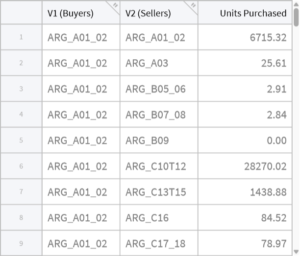
Retrieves OECD SML Dataset for 2017:

In[]:=

cloud2017=CloudObject[

https://www.wolframcloud.com/obj/kaavyamajumder/2017.csv

];retrieved2017=CloudGet[cloud2017]

Out[]=

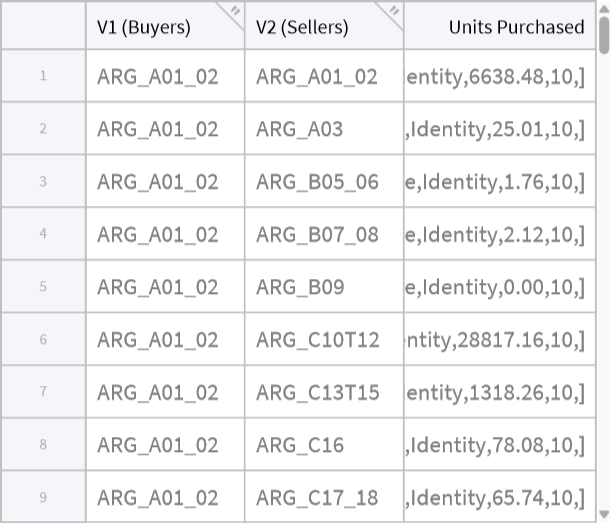
Retrieves OECD SML Dataset for 2018:

In[]:=

cloud2018=CloudObject[

https://www.wolframcloud.com/obj/kaavyamajumder/2018.csv

];retrieved2018=CloudGet[cloud2018]

Out[]=

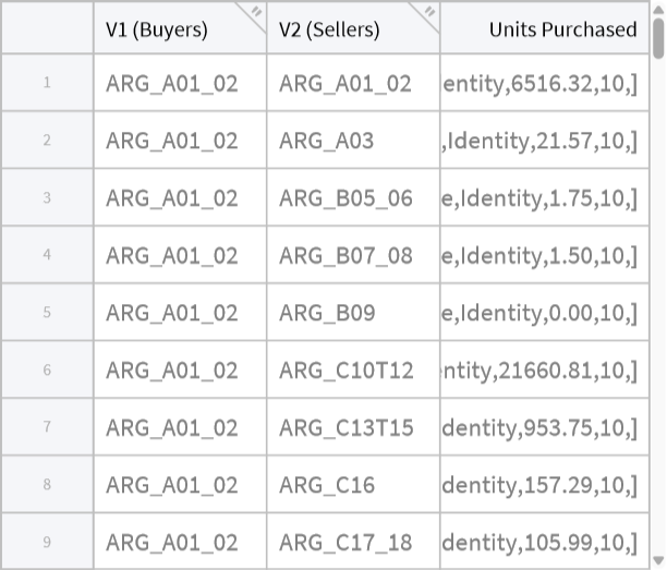
Retrieves OECD SML Dataset for 2019:

Retrieves OECD SML Dataset for 2020:

UNSD Concordances

The UNSD concordance datasets provide official crosswalks between different international classification systems, allowing product- and industry-level datasets that use different coding standards to be linked in a consistent way. In this project, the concordances are used to translate semiconductor-related HS trade codes into the product and industry classifications required for input–output modeling, ensuring that trade-based semiconductor shocks can be aligned with sector-level structures used in the Leontief and Ghosh simulations and make our outputs easier to recreate accurately without mix-ups.

CPC 2.1 <> HS2012

This concordance maps HS 2012 commodity codes to CPC 2.1 product categories. It is used to translate semiconductor HS codes from UN Comtrade into CPC product groups that can be aggregated or filtered consistently before linking them to industry-level data.

Retrieves Concordance Maps for CPC 2.1 <> HS2012:

CPC 2.1 <> HS2017

This dataset performs the same function as the HS 2012 concordance but for HS 2017 classifications, allowing semiconductor trade records reported under newer HS revisions to be mapped to the same CPC 2.1 product framework.

Retrieves Concordance Maps for CPC 2.1 <> HS2017:

CPC 2.1 <> ISIC rev. 4

The next concordance links CPC 2.1 product categories to ISIC Rev. 4 industries. It is used to move from product-level semiconductor classifications to industry-level sectors, enabling semiconductor shocks defined using trade data to be applied to the sectoral structure of the input–output models.

Retrieves Concordance Maps for CPC 2.1 <> ISIC rev.4:

WIOD Socio-Economic Accounts

The WIOD Socio-Economic Accounts provide country- and sector-level economic indicators such as labor inputs, value added, and related socio-economic measures across multiple years. In this project, the SEA data is not used to construct the input–output matrices directly, but to contextualize and interpret the simulation results, helping identify which countries and sectors affected by the semiconductor shock are large employers or major contributors to economic output. This allows the modeled production impacts to be related to real economic scale rather than being interpreted only as abstract network effects.

Retrieves WIOD Socio-Economic Accounts data:

The Ghosh Model

The Ghosh input–output model is a supply-driven framework used to study how changes in sectoral output propagate downstream through an economy. Unlike the Leontief model, which treats final demand as exogenous and traces upstream production requirements, the Ghosh model treats sectoral output as exogenous and examines how reductions in supply affect dependent sectors through fixed output distribution coefficients. Mathematically, the model is based on a matrix of allocation coefficients derived from observed inter-industry transactions, and its inverse captures the total downstream impact of a supply-side shock. The model is constructed from observed inter-industry transaction data by forming a matrix of output allocation coefficients, where each coefficient represents the share of a seller’s total output distributed to a particular buyer. These coefficients encode fixed supply-distribution relationships between sectors.

Let 𝐵 denote the matrix of Ghosh allocation coefficients. The total output response to a supply shock is computed using the Ghosh inverse, given by

where 𝐼 is the identity matrix. This inverse captures both direct effects (immediate buyers of the shocked sector) and indirect effects (buyers of buyers, and so on) as the supply constraint propagates through the production network.In practice, the matrix 𝐼−𝐵 can be ill-conditioned or nearly singular in large empirical input–output systems. To ensure numerical stability, this project computes a stable inverse, which regularizes the inversion process and prevents small numerical errors from producing unrealistic amplification effects. This allows the simulation to remain well-behaved even when working with large, sparse, and highly interconnected transaction networks.

The Ghosh model is particularly relevant for studying upstream disruptions, such as semiconductor shortages, where production constraints originate in a small set of supplying sectors and affect many downstream industries. Because semiconductors function as critical intermediate inputs, a supply shock is more naturally represented as an output constraint rather than a demand reduction, making the Ghosh framework well-suited for this analysis.

Preliminary Calculations and Inverse for 2020

Before running the full simulation across multiple years or introducing sector-specific shocks, we first validate the Ghosh simulation pipeline using OECD SML data for a single year (2020). Restricting the analysis to one year simplifies debugging, ensures that matrix construction and coefficient calculations behave as expected, and allows intermediate outputs to be inspected without the added complexity of cross-year variation. The year 2020 is chosen because it lies within the period of acute global supply disruption and provides a realistic accuracy check and stress-test for the model.

We began by selecting the OECD SML tabular corresponding to the chosen simulation year (2020) and confirms that it has been successfully retrieved as a Tabular object.

Confirms dataset import:

We then extracted the column headers from the SML tabular and explicitly identifies the positions of the buyer, seller, and transaction value columns. We also check whether any of the required columns (buyers, sellers, transaction values) are missing from the dataset. If any column cannot be located, it is flagged explicitly.

Checks for dataset discrepancies:

Next we allow for direct inspection of individual buyer–seller transactions and confirm that each row represents a directed economic link with an associated transaction magnitude.

Converts SML Tabular into row-level associations:

This step extracts the buyer, seller, and transaction value columns from the SML rows into aligned vectors. A length check confirms that each buyer–seller pair is matched with exactly one transaction value.

Extracts relevant columns into aligned vectors:

The buyer, seller, and value vectors are combined into triples representing directed transactions. Entries with zero or non-numeric values are removed, leaving only economically active supply links.

Combines linked vectors and perform imputation of data:

Next, all unique buyers and sellers are collected into a single node set representing country–sector nodes. The size of this set determines the dimension of the Ghosh allocation matrix used in the simulation.

Collates unique buyers and sellers for country-sector nodes:

Then we group the transaction triples by seller and sums all outgoing transaction values to compute each seller’s total sales / total output proxy. The seller count becomes 3903 (down from 3905 nodes in the previous output) because 2 nodes appear only as buyers and never as sellers, so they do not exist as keys in the seller-sum association (the output shows these buyer-only nodes as {TLS, VA}).

Groups transactions by seller:

Finds the buyer-only nodes for confirmation:

We then list the 10 largest sellers by total outgoing transactions in the 2020 SML network. For example, OUT (the Rest of World aggregate that captures transactions with external trading partners outside the explicitly modeled country–sector nodes) has the highest total sales (≈ 172.4 million units), followed by USA_HFCE (≈ 13.0 million) and CHN_F (≈ 7.5 million). These nodes represent the most supply-central country–sector pairs and are expected to generate the largest downstream effects under a Ghosh supply shock.

Lists top 10 largest sellers:

Our next step builds a nested lookup structure of the form seller → (buyer → total purchased from that seller) by first grouping rows by seller, then grouping each seller’s rows by buyer and summing values. This creates a quick and sparse representation of the weighted network that is used next to form allocation coefficients for the Ghosh matrix.

Nested Lookup Structure:

Now, we construct the Ghosh allocation matrix 𝐵 in association form. For each seller, buyer-level transaction totals are divided by the seller’s total sales to compute allocation shares. Each entry represents the fraction of a seller’s output distributed to a specific buyer, implementing:

A check verifies that the allocation shares for a given seller sum to 1, confirming correct normalization. This is required the Ghosh model, since each seller’s output must be fully distributed across its buyers.

Verifies normalization:

We then inspect the distribution of individual allocation shares and network size. The reported minimum and maximum values confirm that shares lie in [0,1], while the counts indicate the number of sellers and the average number of buyers per seller.

Verifies distribution of individual shares and network size:

Next we verify that all sellers’ allocation shares sum to 1 within numerical tolerance. The zero count of deviations confirms that the 𝐵 matrix is well-formed and suitable for computing the Ghosh inverse using:

Verifies seller’s allocation shares:

Here, we identify the top five sellers by total sales in the network. These nodes represent the most supply-central country–sector pairs and are natural candidates for testing downstream propagation in a supply-driven model. We then define the shock vector used in the Ghosh simulation. A −0.2 shock (20% output reduction) is assigned to the top sellers, while all other nodes receive zero. This encodes an exogenous supply contraction consistent with the assumptions of the Ghosh framework.

Identifies top sellers and assign a −20% exogenous supply shock:

This table confirms the shock assignment by listing each shocked seller alongside its total sales and assigned shock value. Applying the same proportional shock across the largest sellers creates a controlled stress test that isolates the effect of network structure, rather than differences in shock magnitude.

Reports baseline output and uniform supply shock for top sellers:

Next we compute the first-round downstream output change: each seller’s shock:

is distributed to its buyers using the Ghosh shares 𝑏𝑖𝑗, then summed across sellers. ghDelta1Full fills missing nodes with 0.

Computes first-round downstream output losses via Ghosh shares:

We then list the largest negative one-step impacts e.g., OUT, USA_L, USA_G and the smallest impacts eg. ARG_HFCE, AUS_NPISH (mostly exact 0, meaning no direct exposure at one step).

Ranks nodes by first-round downstream impact:

This is a check that compares the total one-step impact LHS = Total[ghDelta1Full] to a direct recomputation from shocked sellers RHS. The difference (≈ 2.41×10^6) reflects rounding and network filtering.

Compares aggregated first-round losses to direct shocked-seller calculation:

This counts affected nodes: 3441 have negative one-step impact and 462 are exactly zero.

One-step exposure counts:

We then display the 10 most negative one-step impacts as a table.

Displays most impacted one-step values:

Now, we convert the absolute one-step output changes into relative impacts by dividing each node’s change by its baseline output, ensuring that effects are comparable across nodes of different sizes. Nodes with zero baseline output are assigned a relative impact of zero to avoid undefined values. Outputs show the range of relative impacts across all nodes and identify the country–sector nodes experiencing the largest proportional losses after one downstream propagation step.

Calculates relative first-round Ghosh impacts across nodes:

We compute the one-step updated output for each node by combining its direct shock with the downstream effect it receives from shocked suppliers. Then the cell converts the updated output into a proportional change relative to the baseline output, producing a single interpretable impact measure per node.

Computes one-step updated output and relative total impact:

Here we fix the node ordering for the matrix representation. Each country–sector node is assigned a unique integer index, which is required to convert association-based Ghosh shares into a matrix form.

Defines node index mapping for matrix representation

Next we convert the Ghosh allocation shares into sparse matrix rules of the form (buyer index, seller index → weight) and builds the sparse Ghosh matrix. Using a sparse representation keeps the computation efficient for a large, mostly zero network.

Builds sparse Ghosh allocation matrix:

Then we check column sums of the Ghosh matrix. Columns summing to one confirm correct normalization for seller nodes, while zero-sum columns correspond to nodes that never act as sellers. The output confirms this structure and identifies how many columns fall into each case.

Checks column sums of the Ghosh matrix:

This cell restricts the column-sum check to actual sellers only. The output shows that all seller columns sum to exactly one, confirming that the Ghosh allocation matrix is well-formed and ready for inversion.

Checks Ghosh normalization restricted to sellers:

We then construct numeric vectors for baseline output and shocks in the same node order as the Ghosh matrix and convert percentage shocks into absolute output shocks. This aligns all inputs for matrix-based simulation. Here, the identity matrix is created and the full Ghosh system:

is solved using a sparse linear solver. This computes the total downstream impact, including all higher-order propagation effects captured by the Ghosh inverse.

Computes full-equilibrium Ghosh impact via matrix inversion:

This output converts total output changes into relative impacts and lists the nodes with the largest overall contractions. Unlike the one-step results, these values reflect the full equilibrium effect after the shock propagates through the entire production network.

Next we create ghCompare, which measures how the one-step approximation differs from the full inverse result for each node by subtracting ghImpact (full propagation) from ghImpactOneStep (first-round only). This makes it easy to see where higher-order ripple effects add substantial extra impact beyond direct exposure.

Quantifies difference between one-step and full Ghosh effects:

The helper function ghNumAssoc forces all association values to be numeric (non-numeric values become 0). It is then applied to create ghImpactN and ghCompareN, which prevents formatting or missing-value issues from breaking later summary statistics and tables.

Replaces non-numeric association values with zero:

Here we define ghSummaryRow, which summarizes an impact association using simple diagnostics: minimum, maximum, total sum, number of nodes, and number of zeros. The output for ghImpactN shows the overall range of full-propagation impacts (with the most negative node around −0.674), confirms the network size (3905 nodes), and reports how many nodes have exactly zero impact.

Generates summary statistics for equilibrium impacts:

Here we display ghTopBottomTable, which shows the bottom 𝑛 (most negative) and top 𝑛 (most positive) impacts side by side for quick inspection. The output confirms that the largest effects are strongly negative (e.g., nodes like USA_L, USA_G, and OUT), while the “top” side is essentially zeros, indicating that this shock setup produces contractions but no positive output gains in the model.

Compares bottom and top impacts:

Ghosh Simulation on the Semiconductor Shock

The semiconductor shock during roughly 2018–2022 was a period where upstream chip supply could not meet demand due to capacity constraints, factory shutdowns, logistics bottlenecks, and long lead times in semiconductor fabrication. Because semiconductors are critical intermediate inputs for electronics, automobiles, and industrial equipment, these shortages translated into downstream production disruptions across many sectors. In this section, we apply the Ghosh supply-driven model to represent this event as an exogenous reduction in output for semiconductor-linked suppliers, and we trace how that supply constraint propagates through the buyer–seller transaction network using the Ghosh allocation structure and inverse.

Retrieving data and creating helper functions

We begin by defining the set of years we will iterate over (2016–2020) and create ghGetRetrieved, a helper that fetches the corresponding preloaded SML tabular (e.g., retrieved2020) if it exists, otherwise returning a missing marker. This standardizes year-by-year retrieval without manually referencing each symbol.

Sets analysis years and helper for retrieving yearly SML data:

We create ghToRowAssociations, which converts the tabular into a consistent row-level representation (associations with column keys). This is a formatting step that makes later extraction of buyer, seller, and value columns reliable, even if the internal tabular structure varies slightly.

Standardizes tabular format:

Below we define ghSMLTriplesFromTab, which turns a year’s SML tabular into the clean transaction triples used by the model. It extracts the buyer column (“V1 (Buyers)”), seller column (“V2 (Sellers)”), and transaction values (“Units Purchased”), replaces missing values with 0, and filters to keep only valid triples where buyer/seller are strings and the value is numeric and positive.

Converts yearly SML data into transaction triples:

Creating one-year Ghosh objects

We then build ghBuildYearModel, which builds all core Ghosh objects for a single year from the triple list. It constructs the node set, computes total sales per seller (x0), groups transactions into seller→buyer totals (z), converts these totals into normalized Ghosh shares (b), assigns node indices, and builds the sparse Ghosh matrix (bmat). It then checks column sums and applies a renormalization step so that seller-columns sum to 1, returning a compact package containing the node list, baseline outputs, allocation shares, sparse matrix, and index map for that year.

Constructs yearly Ghosh model from transaction triples:

Building multi-year models

We then create ghSMLTriples, which stores the cleaned buyer–seller–value triples for each year in ghYears. The report table summarizes how many valid transaction triples and unique nodes are available per year, showing that each year has a similar network size (about 3,905 nodes) and millions of nonzero transactions.

Assembles year-wise transaction triples:

Next, we construct ghYearModels by running the one-year builder on each year’s triples. The result is a year → model association, where each model contains the node list, baseline outputs, Ghosh share structure, sparse 𝐵 matrix, and index map for that year.

Builds Ghosh models for each year:

Next we define the function ghCheckYearModel, a validation function that checks whether a year model is internally consistent. It confirms that the matrix is square with the right dimension, that node labels are strings, that the index map matches the node count, that there are no negative nonzero entries, and that seller-column sums behave as expected.

Confirms matrix dimension size for validation:

The code below runs the validation on the 2020 model. The output confirms a 3,905-node square matrix, a valid index mapping, no negative nonzeros, and column sums that range from 0 to 1 (where 0 corresponds to non-seller columns and 1 corresponds to normalized seller columns).

Validates the 2020 Ghosh model:

We produced a compact multi-year diagnostics table by applying ghCheckYearModel to every year model and attaching the year label. The output makes it easy to confirm at a glance that all years have consistent node counts, valid indexing, no negative weights, and correctly normalized seller columns.

Validates all yearly Ghosh models:

We also double-check normalization on the 2020 𝐵 matrix by looking only at active columns (columns with sum > 0, i.e., actual sellers). The output shows there are 3903 active seller columns, and their column sums are essentially exactly 1, with only tiny numerical deviation, confirming the Ghosh share matrix is correctly normalized before inversion.

Rechecks normalization of active seller columns:

Full Ghosh propagation with stable inverse

Now we come to actual propagation and stable inverse of the simulation.
First we define ghMakeSolver, which builds a numerically stable linear solver for the system:

The damping factor 𝜆 makes the inversion more stable for large empirical networks, and the Krylov method is used because it is efficient for sparse matrices.

Builds damped Ghosh solver for stable propagation:

Now we create ghShockVector, which converts a node→shock association into a dense vector aligned with the model’s node index. Values are clipped to stay within valid bounds, ensuring the shock inputs are well-formed before running the solver.

Converts shock association to indexed shock vector:

We then built ghRunShock, which runs the full Ghosh propagation. It builds the baseline output vector from ym[“x0”], creates the solver, and computes a baseline solution and a shocked solution after reducing the exogenous driver for shocked nodes. It then returns the node list along with the baseline outputs, shocked outputs, absolute changes, and percentage changes, which are the core outputs used for interpreting the semiconductor shock impacts.

Runs full Ghosh shock propagation:

Below we convert several retrieved datasets into row-level associations using the same helper (ghToRowAssociations). These include UN Comtrade data for semiconductor-related HS codes (8486, 8541, 8542), UNSD concordance tables (HS–CPC and HS–ISIC), and WIOD SEA data. This standardizes all heterogeneous sources into a common row format for later filtering and aggregation.

Converts datasets into row level associations:

Here are some small helper functions to safely work with inconsistent real-world datasets. ghKeyExistsAnyQ checks whether any expected key exists in a row, while ghPickKey selects the first valid column name from a list of alternatives. ghGetStr safely reads string fields, while ghGetNum converts numeric fields and replaces missing or malformed entries with zero. These are necessary because column names vary across Comtrade vintages and metadata formats and ensure later aggregation steps do not fail due to missing or non-numeric values.

Defines utility functions for safe key lookup and type conversion:

Below is the function ghComtradeAnnualByReporter, which aggregates raw Comtrade rows into annual export totals by reporting country. It detects the correct year, flow direction, reporter code, and trade value columns, filters to valid export rows, and groups values by year and reporter. The result is a clean year → country → export-value structure suitable for computing shocks.

Aggregates Comtrade exports by year and reporting country. Quiet is used here to suppress ToExpression syntax and formatting warnings when year fields are non-numeric. Such invalid year values are explicitly mapped to Missing[“BadYear”]:

Below is ghShockFromComtrade, which constructs a country-level shock vector by comparing exports in a shock year to a base year. For each reporter, it computes the proportional decline in exports and clips the result to the [0,1] range. The output is an association mapping each country to a supply-reduction factor, which can be directly fed into the Ghosh model as an exogenous semiconductor-related output shock.

Constructs country-level shocks from Comtrade export declines:

Next, we compute country-level semiconductor export shocks separately for the three key HS codes (8486, 8541, 8542) using Comtrade data. Each call compares exports in the shock year to the base year and returns a proportional reduction by country. The intermediate error check ensures that any data issues are caught early. The three shock associations are then merged using Max, so each country is assigned its largest observed semiconductor-related export contraction across the three product categories.

Builds combined country-level semiconductor shocks from Comtrade:

We then rank countries by the size of their combined semiconductor shock. It extracts the top affected countries and formats the result as a table showing rank, country code, and shock magnitude in percentage terms. The output highlights countries experiencing near-total export collapses in at least one of the semiconductor categories, which are treated as the strongest upstream supply shocks to be injected into the Ghosh model.

Ranks countries by combined semiconductor shock severity:

Outputs

World Choropleth Map

First we prepare the Comtrade shock data for mapping by cleaning ISO3 country codes and converting them into Wolfram country Entity objects. It builds a reliable ISO3→Entity lookup by automatically choosing the country property that best matches the ISO3 codes present in ghShockCombined, then keeps only the ISO3 codes that appear in both datasets. The output summary confirms what property worked best (here it selects something like a UN/ISO-related code), and reports how many shock codes exist, how many country entities were found, and how many countries overlap and can therefore be plotted.

Quiet is used here to suppress Interpreter/Check warnings when an ISO3 code cannot be interpreted; invalid codes are mapped to Missing[“BadISO”]:

We then visualize the result with a world choropleth map where each country is colored by its shock intensity value. Countries missing from the overlap remain uncolored/neutral, and the legend shows the scale from low shock to high shock. This plot is a quick geographic diagnostic of where the strongest Comtrade-derived semiconductor export contractions are concentrated before feeding shocks into the Ghosh propagation.

Normalizes country codes, safely extracts keys, and coerces ghShockCombined into a consistent association format:

Normalizes and sorts shock data by ISO codes, and retrieves the available country entities and their properties for validation and lookup:

Selects the country property that best matches shock ISO codes and builds ISO-to-country mappings:

Builds ISO-to-country entities, finds common ISO codes with shock data, and prepares aligned lookup rules:

VIsualizes the world choropleth map:

This choropleth shows how the estimated shock intensity varies across ISO3 reporting countries, highlighting clear differences in exposure rather than a smooth regional pattern. What stands out immediately is that high-intensity values are scattered rather than clustered, with some countries showing strong shocks while neighbouring countries appear far less affected, underscoring how trade exposure is shaped more by a country’s role in global supply chains than by geography alone. Several highly integrated economies display relatively elevated values, reflecting their dependence on tightly coupled production and export networks, while others appear lighter despite regional proximity. The grey areas indicate countries for which no usable mapping or data was available after harmonising identifiers, rather than an absence of shock. Taken together, the map shows that the shock is already uneven at the country level before any network propagation occurs, which is significant because it implies that later spillovers in the Ghosh supply-driven model will be governed by how these uneven country-level disturbances transmit through upstream–downstream input–output linkages, rather than by the initial shock magnitude alone.

Histogram

Our next output visualizes the distribution of semiconductor shock fractions across countries using a histogram. Each bar shows how many countries fall into a given shock interval between 0 and 1. The plot makes it clear that many countries cluster near very small shocks, while a non-trivial number experience large shocks close to complete export loss, confirming that the Comtrade-derived shocks are highly uneven and heavy-tailed before being applied in the Ghosh simulation.

Visualizes histogram showing distribution of shock fractions:

This histogram shows the distribution of shock fractions across all country–sector observations, revealing a strongly skewed pattern rather than a symmetric or uniform spread. Most observations are concentrated at very low shock fractions, indicating that for the majority of nodes the initial disturbance is relatively small, while a thinner but clearly visible tail extends toward high values close to one, capturing a subset of countries or sectors that experience disproportionately large shocks. This heavy-tailed structure is important because it highlights heterogeneity in exposure: shocks are not only uneven across countries, as seen in the map, but also uneven in magnitude across the full set of reporting nodes. The coexistence of many small shocks with a few extreme ones suggests that aggregate outcomes will be sensitive to where these large shocks sit in the production network. In the context of the Ghosh supply-driven simulation, this distribution implies that downstream effects are likely to be dominated by a limited number of highly shocked nodes with strong upstream linkages, rather than by the cumulative effect of many mildly affected ones. Overall, the histogram reinforces the idea that shock propagation in the model is shaped by inequality in initial conditions, providing a quantitative backdrop to why network structure and node position matter so much for the resulting spillovers.

Cumulative Distribution

Here, we plot the empirical cumulative distribution function (CDF) of the semiconductor shock fractions across countries. The x-axis shows the shock intensity, while the y-axis shows the fraction of countries with shocks less than or equal to that value. The shape of the curve highlights the uneven distribution of shocks: a large share of countries experience small shocks, while a significant minority face very large contractions, producing a long right tail in the distribution.

Sorts shock values and computes the empirical cumulative distribution positions:

Visualizes empirical cumulative distribution function:

This cumulative distribution function makes the inequality in shock exposure especially clear by showing how quickly the cumulative share rises at low shock fractions and then flattens before climbing again near the upper tail. A large portion of observations accumulates early, indicating that many countries or sectors experience only very small shocks, while the long, gradual slope through the middle reflects a wide dispersion of intermediate impacts rather than a single typical value. The sharp increase near the right end highlights a relatively small group of nodes with very high shock fractions that account for a non-trivial share of the distribution. Read alongside the histogram, this confirms that the shock structure is heavy-tailed instead of being uniform. In terms of the Ghosh supply-driven framework, this shape matters because it implies that a small fraction of highly shocked nodes sits in the upper tail and can disproportionately influence downstream outcomes once shocks are propagated through input–output linkages. The CDF therefore clarifies not just how unequal the initial shocks are, but why the subsequent network simulation is sensitive to the position and connectivity of these extreme cases rather than to the average level of disruption.

Bmat Heatmap

For our last output we select the year being analysed, extract its Ghosh output matrix (Bmat), and identify the 25 most influential nodes based on column sums, meaning nodes that distribute the most output to others. This builds a 25×25 submatrix containing only these highly active nodes, generates readable labels for them, and ensures the matrix is square and consistent. The heatmap visualises the strength of interdependencies among the top-25 nodes. Brighter colors indicate stronger output linkages, revealing which nodes act as major hubs in propagating shocks through the network. This plot helps identify structurally important sectors or countries where shocks are most likely to amplify and spread across the global production system.

Selects the active year and extracts its Ghosh model, B matrix, and node list for visualization:

Determines the matrix size and derives readable node labels from the available node metadata:

Computes the matrix size and robustly extracts node labels from different possible node formats:

Extracts the active submatrix, selects corresponding labels, and builds axis ticks for plotting:

Visualizes Bmat heatmap:

This heatmap visualises the structure of the B matrix from the Ghosh supply-driven model, restricted to the top 25 most active nodes selected by column sums, and it reveals a highly uneven pattern of interdependence within the production network. Most cells remain relatively muted, indicating that for many pairs of sectors the direct supply-driven influence is weak, while a small number of bright, concentrated patches stand out as hotspots of strong dependence. These hotspots signal specific seller–buyer relationships where a supply shock in one node would disproportionately transmit downstream to others, highlighting structural bottlenecks rather than broad, diffuse connectivity. The fact that intensity is clustered along particular rows and columns rather than spread evenly suggests that influence in the Ghosh framework is asymmetric, with a few key sectors exerting outsized leverage over the system. The concentration of the strongest values along the diagonal reflects high self-dependence of these sectors, meaning shocks initially reinforce themselves within the same node before spreading through the network. In practical terms, this implies that internal sectoral structure plays a critical role in amplifying or dampening shocks in the Ghosh simulation, even before cross-sector spillovers become important. This pattern reinforces the interpretation of the earlier shock maps and distributions: shocks do not propagate uniformly, but are filtered and amplified through a sparse set of dominant linkages embedded in the B matrix. In the context of the Ghosh simulation, this heatmap shows the mechanical channels through which initial country- or sector-level shocks can cascade, making it clear that systemic vulnerability arises less from average connectivity and more from these concentrated structural dependencies.

Interpretation of the Ghosh Results

Taken together, these results show how the Ghosh supply-driven model translates uneven initial shocks into structured, network-dependent outcomes rather than diffuse, average effects. The choropleth establishes that shock intensity is already highly heterogeneous across countries, shaped by their positions in global production networks rather than geography, while the histogram and empirical CDF demonstrate that this heterogeneity is strongly skewed, with many nodes experiencing negligible shocks and a small but important subset facing extreme ones. The B-matrix heatmap then reveals the mechanism behind this behaviour: supply dependencies are sparse and asymmetric, concentrated in a limited set of dominant nodes and self-reinforcing diagonal structures that act as amplification points. Read together, these visualisations tell a coherent story in which the Ghosh model does not simply propagate shocks proportionally, but filters them through unequal initial conditions and concentrated structural linkages, making downstream impacts disproportionately sensitive to where large shocks originate and how tightly those nodes are embedded in the input–output network.

References

United Nations Statistics Division. (n.d.). Correspondence tables (including CPC ↔ HS). UNSD Classifications. https://unstats.un.org/unsd/classifications/Econ

UN Comtrade. (n.d.). UN Comtrade data access / API (download of trade data). https://comtradeplus.un.org/TradeFlow

OECD. (n.d.). Inter-Country Input-Output (ICIO) Tables (data and documentation). https://www.oecd.org/sti/ind/inter-country-input-output-tables.htm

World Input-Output Database (WIOD). (n.d.). WIOD data (including Socio-Economic Accounts / SEA, where provided). https://www.rug.nl/ggdc/valuechain/wiod/

Ghosh, A. (1958). Input-Output Approach to an Allocation System. Economica, 25(97), 58–64. https://www.jstor.org/stable/2550694

Miller, R. E., & Blair, P. D. (2022). Input-Output Analysis: Foundations and Extensions (3rd ed.). Cambridge University Press. https://www.researchgate.net/publication/44529797_Input-output_analysis_foundations_andextensions_Ronald_E_Miller_Peter_D_Blair

Oosterhaven, J. (1988). On the Plausibility of the Supply-Driven Input-Output Model. Journal of Regional Science, 28(2), 203–217. https://onlinelibrary.wiley.com/doi/abs/10.1111/j.1467-9787.1988.tb01208.x

Dietzenbacher, E. (1997). In vindication of the Ghosh model: A reinterpretation as a price model. Journal of Regional Science, 37(4), 629–651. https://onlinelibrary.wiley.com/doi/abs/10.1111/0022-4146.00073

Acemoglu, D., Carvalho, V. M., Ozdaglar, A., & Tahbaz-Salehi, A. (2012). The Network Origins of Aggregate Fluctuations. Econometrica, 80(5), 1977–2016. (Working paper version). https://economics.mit.edu/sites/default/files/publications/The%20Network%20Origins%20of%20Aggregate%20Fluctuations.pdf

Carvalho, V. M. (2014). From Micro to Macro via Production Networks. Journal of Economic Perspectives, 28(4), 23–48. https://www.aeaweb.org/articles?id=10.1257/jep.28.4.23

Inoue, H., & Todo, Y. (2019). Firm-level propagation of shocks through supply-chain networks. PLoS ONE, 14(3), e0213675. https://www.researchgate.net/publication/335133551_Firm-level_propagation_of_shocks_through_supply-chain_networks

Acknowledgements

First and foremost, we’d like to thank our mentor, Carlos Angulo, for constantly guiding us, checking in on us, and helping us out when we were stuck. This essay would have been incomplete without his invaluable insights and inputs. We’d also like to thank the program directors, Rory and Eryn, for giving us the opportunity to participate in this amazing program, and for always keeping us on track and accountable and pointing any technicalities. Lastly, we’d like to thank our previous mentors and all the TAs at WSRP who taught us all we needed to know and instilled a passion for Wolfram in us!

CITE THIS NOTEBOOK

Simulating semiconductor supply shocks in global production networks
by Kaavya Majumder, Sarim Mominkhawaja, Adit Amit Kumar, and Rakhi Jain
Wolfram Community, STAFF PICKS, February 11, 2026
https://community.wolfram.com/groups/-/m/t/3638626