Overview
Overview
Sometimes inconsistent, intuitive observations generate interesting discoveries and stimulate exploration.
As the kids say, "I was just playing" with the function ConcaveHullMesh, and suddenly got complex and beautiful 2D and 3D structures:
As the kids say, "I was just playing" with the function ConcaveHullMesh, and suddenly got complex and beautiful 2D and 3D structures:

Utilites
Utilites
To save space, all results here are presented as plain images. For to get graphics output please run code with Mathematica (for 3D examples it may take up to minute).
◆
Clear[rndPoints,cuboidPoints,sectPoints,showData2D,showData3D];(*Randompointsinunitcuboid*)rndPoints[num_,dim_]:=RandomPoint[Cuboid[Array[0&,dim],Array[1&,dim]],num];(*Selectpointsincuboidwithvertexp1andsizedinscaledcoordinates*)cuboidPoints[pts_,p1_,d_]:=With[{cb=CoordinateBounds@pts},{rf=MapThread[Rescale[#1,{0.,1.},#2]&,{#,cb}]&},{wnd=Cuboid[rf@p1,rf@p1+d(cb[[1,2]]-cb[[1,1]])]},{rm=RegionMember@wnd},{wnd,Select[pts,rm]}];(*Selectpointsnearesttogivenplanepassingthroughthepoint{0.5,0.5,h}inthedirectionsϕ,θ*)sectPoints[pts_,ϕ_,θ_,h_,δ_]:=Block[{df=RegionDistance@InfinitePlane[{0.5,0.5,h},{{1,Cos[ϕ],Sin[ϕ]},{1,Cos[θ],Sin[θ]}}]},Select[pts,df@#<δ&]];showData2D[pts_]:=Graphics[{PointSize@0.002,Opacity@.4,StandardBlue,Point@pts},ImageSize->200];showData3D[pts1_,ps1_:0.001,pts2_:{},ps2_:0.]:=Graphics3D[{PointSize@ps1,Opacity@.1,StandardBlue,Point@pts1,PointSize@ps2,Opacity@.8,Orange,Point@pts2},Boxed->False,ImageSize->250];SetOptions[ConcaveHullMesh,PerformanceGoal->"Speed"];SetOptions[MeshRegion,MeshCellStyle{0->Directive[PointSize@0.005,StandardBlue]}];
Introduction
Introduction
Not quite strictly we can define α-shape (or α-complex, or concave hull) as subset of Delaunay triangulation, whose elements are contained in a ball of radius at most without including other points:
α
Block[{pts=rndPoints[33,2]},Row[Labeled[ConcaveHullMesh[pts,#],"α = "<>ToString@#]&/@{0.1,0.15,0.25}]]
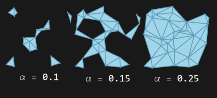
A more precise and detailed definition can be found here. Built-in Mathematica ConcaveHullMesh provides great capabilities for generating α-shapes of any dimensions.
Main module
Main module
With Lloyd relaxation process in mind, I decided to explore the next iterative algorithm. Starting with a set of random points, find their concave hull of a given dimension and determine the centroids for all cells of hull. These will be our new points, for which we find again concave hull etc. It turned out that the most interesting results are obtained if in the process of iterations we change α-parameter. Here is a module for such an algorithm.
isList: list of iteratioins or last result
numIters: number of iterations
initPts: initial points
initK: initial index of iterations
dimCell: dimension of centroids
dimMesh: dimension of concave hull
alphaFunc: law of change α-parameter on iteration index (as pure function)
isList: list of iteratioins or last result
numIters: number of iterations
initPts: initial points
initK: initial index of iterations
dimCell: dimension of centroids
dimMesh: dimension of concave hull
alphaFunc: law of change α-parameter on iteration index (as pure function)
In[]:=
Clear@nestConcaveMesh;nestConcaveMesh[isList_,numIters_,initPts_,initK_,dimCell_,dimMesh_,alphaFunc_]:=Block[{k=initK,head=If[isList,NestWhileList,NestWhile]},head[(k++;ConcaveHullMesh[AnnotationValue[{#,dimCell},MeshCellCentroid],alphaFunc@k,dimMesh])&,(*Initialregion*)ConcaveHullMesh[initPts,alphaFunc@initK,dimMesh],(*Testifdegenerate*)MeshRegionQ,1,numIters]];(*Onlypoints(0-cells)oflastiteration*)Clear@nestConcavePts;nestConcavePts[numIters_,initPts_,initK_,dimCell_,dimMesh_,alphaFunc_]:=Block[{k=initK},NestWhile[(k++;AnnotationValue[{ConcaveHullMesh[#,alphaFunc@k,dimMesh],dimCell},MeshCellCentroid])&,initPts,!SameQ[#,{}]&,1,numIters]];
Signature of examples:
〈 Embedded Dimension, ConcaveMesh Dimension, Centroid Dimension 〉
〈 Embedded Dimension, ConcaveMesh Dimension, Centroid Dimension 〉
Main result for 〈 2, 1, 1 〉
Main result for 〈 2, 1, 1 〉
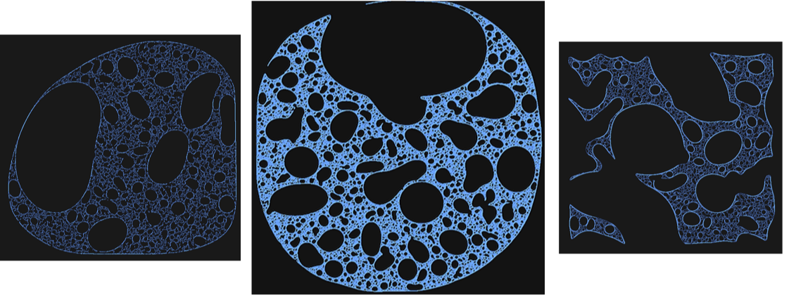
Let’s study the simplest case: 2D points, 1D concave mesh and centroids of 1D cells. Let’s reduce α-parameter in the process of iterations. Try the power and exponential laws.
In[]:=
RownestConcaveMeshTrue,40,rndPoints[30,2],0,1,1,0.3*&[[;;;;8]]
(1+#)
0.9

In[]:=
RownestConcaveMeshTrue,80,rndPoints[30,2],0,1,1,0.6(1+)&[[;;;;15]]
0.75
#

Dive into fractal
Dive into fractal
Take a result of large enough number of iterations:
In[]:=
alphaF=0.3*&;numInitIters=50;numStepIters=20;res=nestConcavePts[numInitIters,rndPoints[50,2],0,1,1,alphaF];showData2D@res
(1+#)
0.92
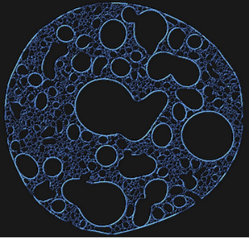
Using the function cuboidPoints we can cut out a small square, and continue the iteration for it.
The scaled coordinates and the size of the square should be chosen manually in a non-empty area. This applies to all other examples.
The scaled coordinates and the size of the square should be chosen manually in a non-empty area. This applies to all other examples.
As with any fractal, this process will be exciting self-similar.
In fact one can use different laws of change α-parameter, different initial configurations of points - the results will be quite similar. I am convinced that these are fractals, but unfortunately so far no one has been able to help me understand the mathematical nature of these results.
In fact one can use different laws of change α-parameter, different initial configurations of points - the results will be quite similar. I am convinced that these are fractals, but unfortunately so far no one has been able to help me understand the mathematical nature of these results.
Another dimensions
Another dimensions
The main problem for other dimensions is a much greater sensitivity to the initial data and changes α-parameter. In most cases, the resulting structures either tend to convex hull or degenerate. However, it was possible to find the conditions under which non-trivial structures are obtained. But to identify them in more detail, studies with a much larger number of points are needed.
〈 2, 1, 2 〉
〈 2, 1, 2 〉
I find it difficult to recognize this structures. In this case the law of change α-parameter does not play a special role, it is just that when too fast reduction occurs decay. It looks like not fractal, but something unusual.
Just magnification
〈 3, 1, 1 〉
〈 3, 1, 1 〉
If we iterate 1D mesh in 3D space, then most often will be obtained convex hull or some fragmented structures. But there is a wide range of parameter change laws, in which the resulting sets have a beautiful unusual structure and in the sections clearly demonstrate fractals.
Rotation angles and position of section plane in sectPoints should be chosen manually for to get non-empty result. This applies to all other examples.
Rotation angles and position of section plane in sectPoints should be chosen manually for to get non-empty result. This applies to all other examples.
〈 3, 2, 3 〉
〈 3, 2, 3 〉
This combination of dimensions gives rise to fragmented structures, which are unlikely to be fractals but are of interest for possible studies.
What next
What next
In the near future, I’m going to implement an efficient algorithm for calculation multi-fractal dimension in Mathematica, and apply it to the results. Of interest is also the case 〈 1, 1, 1 〉, as possible generalization of Cantor set. Of course, I would like professional mathematicians to pay attention to these observations and suggest possible explanations.
CITE THIS NOTEBOOK
CITE THIS NOTEBOOK
Exploring α-shapes with Wolfram
by Denis Ivanov
Wolfram Community, STAFF PICKS, January 11, 2026
https://community.wolfram.com/groups/-/m/t/3604256
by Denis Ivanov
Wolfram Community, STAFF PICKS, January 11, 2026
https://community.wolfram.com/groups/-/m/t/3604256