Introduction to the TSP
Introduction to the TSP
The Traveling Salesman Problem is a famous computational complexity theory problem. It consists in finding the shortest path connecting a number of cities, that allows the salesman to visit each city once and return to the origin city. Different versions of the problem have allowed a variety of solutions to be developed, each presenting perks and downsides, making some solutions more adapted to the studied issue than others.
Our goal with this project
Our goal with this project
We chose to adapt the TSP to one situation in particular : a theme park. Our program should therefore take into account the following variables :
◼
Coordinates of the attraction
◼
Waiting time (popularity,...)
◼
Time of attraction
◼
Time of the day
◼
Wether the day of the visit is on a holiday or on the weekend
◼
The passage of time (the waiting times vary over time)
Different possible methods
Different possible methods
Brute force
Brute force
As mentioned earlier, the TSP has a number of solutions proposed for it. One of the first we came across was Brute Force. It consists in generating each path, or ordering of the points (a permutation of the different points entered into the program), calculating the duration of the route tested, and returning the path with the shortest journey route. This came across as a good way to solve our problem, as it is certain to find the shortest path (the most optimal solution), as it is the easiest to code and as it allows to add every variable we wanted.
Here is an example of the use of Brute Force:
In[]:=
Clear[f]points={{0,0},{1,0},{2,1},{1,2},{2,2},{0,1}};f[s_]:=First[Sort[Table[{n,Total[ResourceFunction["AppendSequence"][Table[Norm[Part[n,a]-Part[n,a-1]],{a,2,Length[s]}],Norm[Part[n,1]],Norm[Part[n,Length[s]]]]]},{n,Permutations[s]}],#1[[2]]<#2[[2]]&]]f[points]finpoints=Prepend[Append[points,{0,0}],{0,0}]fleches=Table[Arrow[{finpoints[[i]],finpoints[[i+1]]}],{i,1,Length[finpoints]-1}];labels=Table[Text[Style[Row[{i-1,": ",finpoints[[i]]}],12,Bold,Black],finpoints[[i]],{1.5,0}],{i,1,Length[finpoints]}];Graphics[{Thick,Arrowheads[0.03],fleches,Black,PointSize[Large],Red,Point[finpoints],labels},Axes->True,AxesOrigin->{0,0}]
Out[]=
{{0,1},{1,2},{2,2},{2,1},{1,0},{0,0}},4+2
2
Out[]=
{{0,0},{0,0},{1,0},{2,1},{1,2},{2,2},{0,1},{0,0}}
Out[]=
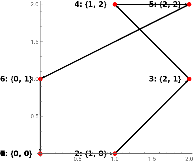
However, its major disadvantage was its computational weight. As it tests every single path, it cannot be used for more than 8 attractions, because the code becomes very heavy to execute.
FindShortestTour
FindShortestTour
We found numerous Wolfram functions, such as FindShortestTour, which takes a point and returns the next nearest point. Though this solution allowed us to optimize the distance and to create a cycle, we quickly realised that it would be difficult to add all of our variables.
Here is an example of the use of FindShortestTour:
In[]:=
list={{1,2},{6,3},{2,3},{0,6},{7,5},{9,3},{5,1},{4,4},{7,7}};path=FindShortestTour[list];ListLinePlot[Table[list[[path[[2]][[i]]]],{i,Length[list]+1}],Frame->True,GridLines->Automatic]
Out[]=
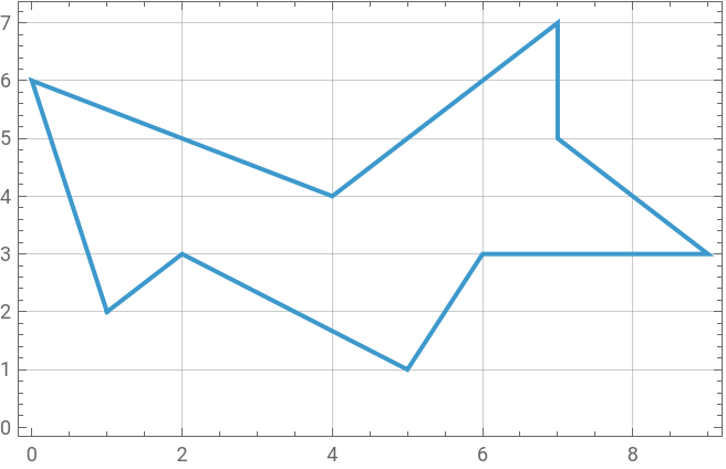
However, we could not use these functions, as they only take into consideration distance, and we wanted to able to add our own variables, on which the shortest path depends.
Dijkstra and Bellman-Ford
Dijkstra and Bellman-Ford
We then considered using a Dijkstra or Bellman-Ford algorithm, which rely on graph theory to find the shortest path from a point A to a point B, with a weight associated with each edge of the graph. These algorithms calculate a large number of routes at the same time and decide which way is worth continuing. As we could modify the coefficient of the edges, we could therefore integrate our variables. However, on of the main points of this project was creating a cycle, and these algorithms focus on getting from a point to another point of the plane, they were did not correspond to our criteria.
Nearest Neighbour
Nearest Neighbour
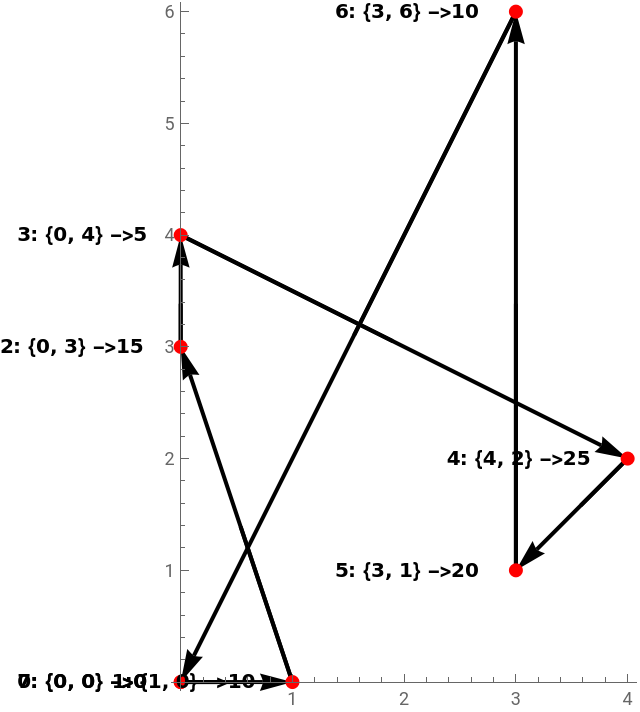
We thought about the Nearest Neighbor approach, which is that at a given point, the algorithm searches for the next nearest point, adds it to a list, and continues, until having finished visiting, all of the points. We were able to create a cycle and to add the waiting time and we could have added more variables. However, we quickly noticed that the problem is that it is not at all optimal, as the nearest point B to a point A, isn’t necessarily to point C, and another arrangement might be more optimal.
Here is an example of the use of Nearest Neighbour:
In[]:=
Clear[f,g,liste,path,total,arrows,labels]g[list_]:=Module[{unvisited=list,path={},current={0,0},next,cost,total=0,best},While[Length[unvisited]>0,best=First[SortBy[Table[{Norm[pt[[1]]-current]+pt[[2]]+Norm[pt[[1]]],pt},{pt,unvisited}],First]];{cost,next}=best;AppendTo[path,next[[1]]];total+=Norm[next[[1]]-current]+next[[2]];current=next[[1]];unvisited=DeleteCases[unvisited,next];];total+=Norm[current];{path,total}];list={{{0,4},5},{{1,0},10},{{3,1},20},{{4,2},25},{{0,3},15},{{0,0},5},{{3,6},10}};{path,total}=g[list];fullPath=Append[path,{0,0}];arrows=Table[Arrow[{If[i==1,{0,0},fullPath[[i-1]]],fullPath[[i]]}],{i,1,Length[fullPath]}];labels=Table[Module[{wait},wait=If[fullPath[[i]]==={0,0},0,SelectFirst[list,#[[1]]===fullPath[[i]]&,{_,0}][[2]]];Text[Style[Row[{i-1,": ",fullPath[[i]]," ->",wait}],10,Bold,Black],fullPath[[i]],{1.5,0}]],{i,1,Length[fullPath]}];Graphics[{Thick,Arrowheads[0.07],arrows,Black,PointSize[Large],Red,Point[Prepend[path,{0,0}]],labels},Axes->True,AxesOrigin->{0,0}]
Out[]=
Genetic algorithms
Genetic algorithms
Concept
Concept
A genetic algorithm is a form of optimisation inspired by natural selection : the first step is to create a population composed of a sample of permutations, which are different routes (because we are looking for the most optimal route, they are potential answers to the problem). Then, we evaluate them, by assigning them a score that is calculated by an preestablished function, called the “fitness function”. Like with natural selection, only the best answers are are retained. The next generation is generated through random mutation and combination of couples of “parents”, to preserve diversity, and prevent getting stuck in loops that test and reproduce the same routes repeatedly. The process is repeated hundreds of times, at the end of which we find the most optimal solution amongst the ones tested.
This turned out to be the most optimal solution for us, as it could test however we wanted the paths, like Brute Force, but without generating every function.
This turned out to be the most optimal solution for us, as it could test however we wanted the paths, like Brute Force, but without generating every function.
The part of the algorithm responsible for creating the next generation :
child=Table[Module[{p1,p2,cut1,cut2,sons,remaining},{p1,p2}=RandomSample[survivors,2];{cut1,cut2}=Sort[RandomInteger[{1,numPoints},2]];sons=Take[p1,{cut1,cut2}];remaining=DeleteCases[p2,Alternatives@@sons];Join[Take[remaining,cut1-1],sons,Drop[remaining,cut1-1]]],{Length[survivors]}];
Parameters of the genetic algorithm
Parameters of the genetic algorithm
In our case, our potential solutions are combinations of the different attractions. We had already chosen the number of random solutions that will compose our original population, which is 50, the number of generations, 200 and the mutation probability, which is 20%. We started by entering the amount of attractions and their coordinates, and we created the first generation.
numperm=50;numgeneration=100;probmutation=0.2;numPoints=Length[list];
Fitness function
Fitness function
Each generation is evaluated using a score assigned to each attraction by the fitness function, which takes into account the variables we have chosen. The longer the path, the higher the score and the less likely the solution is to be chosen.
The fitness function is used to evaluate a route, meaning an ordering of the attractions to visit. It calculates a score, which in this case is the total time required to make the path. This score allows us to compare how efficient one route is compared to another.
The function takes as input the list of attractions, along with their information, such as popularity and duration. To simulate the attraction duration, we created a function (g[x]) that produces a coefficient based on the time spent at each attraction. The longer the duration of the attraction, the higher the coefficient will be. We also included two additional coefficients: one for whether the visit is on a holiday, and another for whether it is on a weekend.
Both factors influence how crowded the park is, which increases the waiting time for attractions. Another function (f[x]) simulates how waiting times vary throughout the day. To obtain this function, we took points that associate a coefficient with a time and created the function using Wolfram’s Interpolation tool. For example, there will be fewer people in the queues at 12 noon than at 3 pm due to the lunch break.
Our algorithm also takes into account the time we enter the park. If the planned route goes past the park’s closing time of 7 pm, the algorithm returns “impossible.”. Which means that the route does not allow to make all the attraction in the given time.
At the end, we want to calculate the total duration of a route, and two elements must be considered:
At the end, we want to calculate the total duration of a route, and two elements must be considered:
◼
The waiting time at each attraction at a given moment, which depends on multiple factors.
◼
The travel distance between two attractions.
In order to calculate the total duration, we need to convert travel distance into time. We assumed an average walking speed of 5 km/h, which means that 100 meters = 1.2 minutes. With this conversion, the program can use time as a variable, while still allowing the user to enter attraction positions in terms of distance coordinates.
Final function
Final function
With all these elements that allow us to structure our algorithm and variables, we obtain the following code, which is our final function.
Thorpe park application
Thorpe park application
We decided to provide you with an example, which is our inspiration, Thorpe Park. We added a Grid to the map, and the ability to have coordinates of a point just by clicking on it, to facilitate the process. We chose 10 attractions and looked up their popularity and time length.
We decided to start at 9, the opening of the park, to be sure to be able to do everything and our algorithm gave us this path.
Since we applied our algorithm to this example, it can also be applied to any theme park and even any situation, which is the strength of our code.
CITE THIS NOTEBOOK
CITE THIS NOTEBOOK
The travelling salesman problem: How to find the fastest route through a theme park
by Constance Carlot, Lucie Dilouya and Luisa Laffite
Wolfram Community, STAFF PICKS, September 30, 2025
https://community.wolfram.com/groups/-/m/t/3552881
by Constance Carlot, Lucie Dilouya and Luisa Laffite
Wolfram Community, STAFF PICKS, September 30, 2025
https://community.wolfram.com/groups/-/m/t/3552881