While looking at polynomials, one quickly realises that a polynomial can be written in multiple ways. As the polynomials size increases so does the possibilities of that polynomial’s transformations. When one says transformation for polynomials, it isn’t limited to just expanding them, but rather if one were to choose different parts of that polynomial and apply rules of transformation on them. Going on path one can quickly understand that a complex looking polynomial can hence be represented by a simple polynomial of the same family which can be found if enough transformations are done on it.
Introduction
Introduction
We begin by looking at a given polynomial.
In[]:=
poly=(x+3)(x-10)/(x-3);
We can look at the tree-form of the polynomial to better understand the structure of the polynomial.
In[]:=
tf=TreeForm[poly]
Out[]//TreeForm=
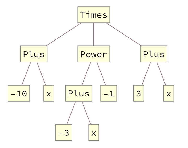
As we can see that a given polynomial is divided into multiple headings based on the operations in the polynomial.
Function on polynomial sub-grouping
Function on polynomial sub-grouping
To create transformations of this polynomial, we created a function that goes along Full Form of the polynomial and tries to group different parts of the polynomial and apply a transformation like Expand or Factor on them. Thus, we can find different transformations of the same polynomial
In[]:=
expressionsFrom[parent_,func_]:=Module[{head,integersubsets,subsets,complements,results},If[Length[parent]==0,Return[{parent}]];head=parent[[0]];If[head===Power,results={func[parent]},integersubsets=Subsets[Range[Length[parent]]];subsets=parent[[#]]&/@integersubsets;subsets=func/@subsets;complements=Complement[Range[Length[parent]],#]&/@integersubsets;complements=parent[[#]]&/@complements;results=MapThread[head[#1,#2]&,{subsets,complements}];];DeleteCases[Union[results],parent]];
An example of various transformations that can happen on our above chosen polynomial is displayed below.
In[]:=
expressionsFrom[poly,Expand]
Out[]=
(3+x)-+,(-10+x)+,,--+
10
-3+x
x
-3+x
3
-3+x
x
-3+x
-30-7x+
2
x
-3+x
30
-3+x
7x
-3+x
2
x
-3+x
Multiway System
Multiway System
After creating a function that choses grouping of various parts of the polynomial, we created a multiway system to see how the polynomial transformed.
The multiway system was created by using the NestGraph function inbuilt in Mathematica. The function applies a given function on a starting node, ie parent, and then applies successively on the children and sub-children n times as defined.
The multiway system was created by using the NestGraph function inbuilt in Mathematica. The function applies a given function on a starting node, ie parent, and then applies successively on the children and sub-children n times as defined.
In[]:=
NestGraph[expressionsFrom[#,Expand]&,poly,3]
Out[]=
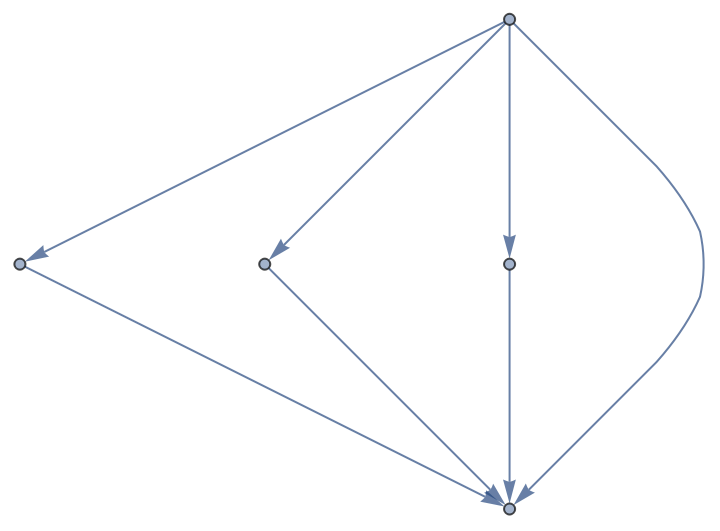
Similarly when another transformation, Factor was also applied to the polynomial, and levels increased from 3 to 4, the system evolved to this.
In[]:=
nn=NestGraph[Join[expressionsFrom[#,Expand],expressionsFrom[#,Factor]]&,poly,4,VertexLabelsAutomatic]
Out[]=
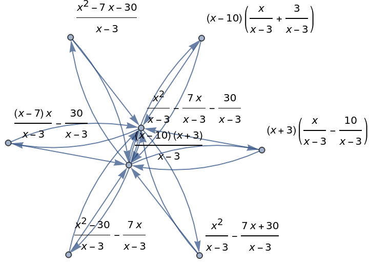
This is our multiway system that shows us possible transformations of the polynomial under our given rules.
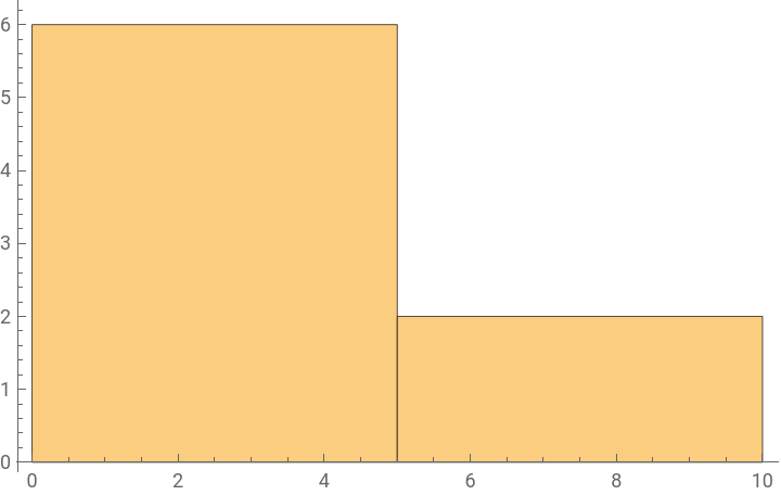
We can look at various metrics of the graph like number of vertices and edges, plot the number of incoming and outgoing edges from those vertices and see the distributions.
We can look at various metrics of the graph like number of vertices and edges, plot the number of incoming and outgoing edges from those vertices and see the distributions.
In[]:=
vertexcount=VertexCount[nn]Incoming=CountsBy[EdgeList[nn],Last];ik=Keys[Incoming];incomingedgespervertex=Values@Incoming
Out[]=
8
Out[]=
{1,1,1,7,7,1,1,1}
In[]:=
outgoing=CountsBy[EdgeList[nn],First];ok=Keys[outgoing];outgoingedgespervertex=Values@outgoing
Out[]=
{4,2,2,2,4,2,2,2}
In[]:=
Histogram[incomingedgespervertex,PlotRangeAll]Histogram[outgoingedgespervertex,PlotRangeAll]
Out[]=
Out[]=
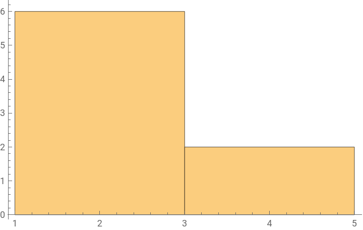
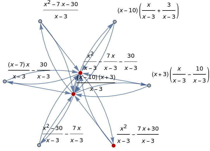
Here we have tried to highlight the parent and the vertex with highest edges coming out of it.
In[]:=
FindShortestPath[nn,poly,ik[[Max[Values@Incoming]]]]HighlightGraph[nn,PathGraph[%]]
Out[]=
,--+,-
(-10+x)(3+x)
-3+x
30
-3+x
7x
-3+x
2
x
-3+x
2
x
-3+x
30+7x
-3+x
Out[]=
One way to do expression simplification from the given graph is to look for Leaf Count of the various vertices of the graph. Leaf Count counts the length of the expression and one definition of simplification, in our case, can be the length of the polynomial. If the polynomial can be written in its shortest form, we can consider it to be simplified, no matter the algebraic form.
In[]:=
lf=LeafCount/@VertexList[nn]maxlf=Max[lf]minlf=Min[lf]maxlfpos=Position[LeafCount/@VertexList[nn],maxlf][[1,1]]minlfpos=Position[LeafCount/@VertexList[nn],minlf][[1,1]]maxlff=VertexList[nn][[maxlfpos]](*BiggestForm*)minlff=VertexList[nn][[minlfpos]](*SimplestForm*)
As we can see that we found the Maximum and minimum Leaf Count of vertices, we have, according to our definition, found the simplest and biggest form of polynomial. Now we can highlight those points and try to find a path between them.
Recursive Function
Recursive Function
Our old function expressionsFrom works well, but still suffers from limitations, one of which is that it still deals in the heads as seen in Tree Form of the polynomial and isn’t recursive to include subheads.
replaceAllParts recurses on the expression’s subheads and creates more groupings that could be missed by the original expressionsFrom function. This serves as a improvement over expressionsFrom. We chose another polynomial example to rerun our analysis.
And we applied our original expressionsFrom function on it.
Once we include our recursive function, the system evolves to this.
We can clearly see how many more transformations were possible once the recursive function was included.
After a while the graphs get too big for plotting.
A Check
We conducted a check on the system to ensure that the polynomials in the family are still the same polynomial, by assigning a value to the polynomial and evaluating it.
As the values of random sample of vertices remain the same, we can conclude that the vertices of graph still represent the same polynomial.
Conclusion
Conclusion
The project implements a multiway system on a family of polynomials, resulting in the graph showing the transformations possible on the chosen polynomial. We can then try to find the leaf counts of the vertices to find the simplest version of the polynomial, basing on the assumption that the simplest polynomial is the shortest one in length.
Although it might appear that the expressions with maximum leaf count and/or minimum leaf count are the polynomial forms chosen at the beginning, but that is the consequence of intelligent choosing of polynomial . This multiway system is true and same for all the vertices in the graph, so if one chooses another vertex as the parent polynomial, the graph will be reproduced, with the expressions with maximum leaf count and/or minimum leaf count as same but are now not the originally chosen polynomial.
Future Work
This project was an exploratory project, with a lot of scope for future work to be done. Since the current rules were just using the Mathematica’s inbuilt functions of Factor and Expand, we can try to include more intelligent rules based on pattern matching on different parts of polynomial like difference of squares, completing the squares and so forth. Such rules can give us more possibilities in the multiway system.
Another planned future work is to apply a reinforced learning model on the system. Since multiway system offers us a lot of possible solutions, ie there are expressions with similar Leaf Counts, we can try to train a model that would give us a vertex that we desire, for example in a textbook solution of a polynomial’s transformation would be one of the members of the multiway system, and to zero in on that we can the model.
Trends on histograms about the incoming and outgoing edges per vertex should be investigated as well and might hold some promise.
Keywords
Keywords
◼
Polynomials
◼
Multiway System
◼
Algebraic Transformations
◼
Polynomial Simplification
◼
Expression Simplification
Acknowledgement
Acknowledgement
I would like to thank my mentor Jesse Galef for his amazing help and support during the project, from providing ideas to working out the code with me. I would also like to thank my TA, Swastik Banerjee for agreeing to meet at odd hours to help me with troubleshooting the code.