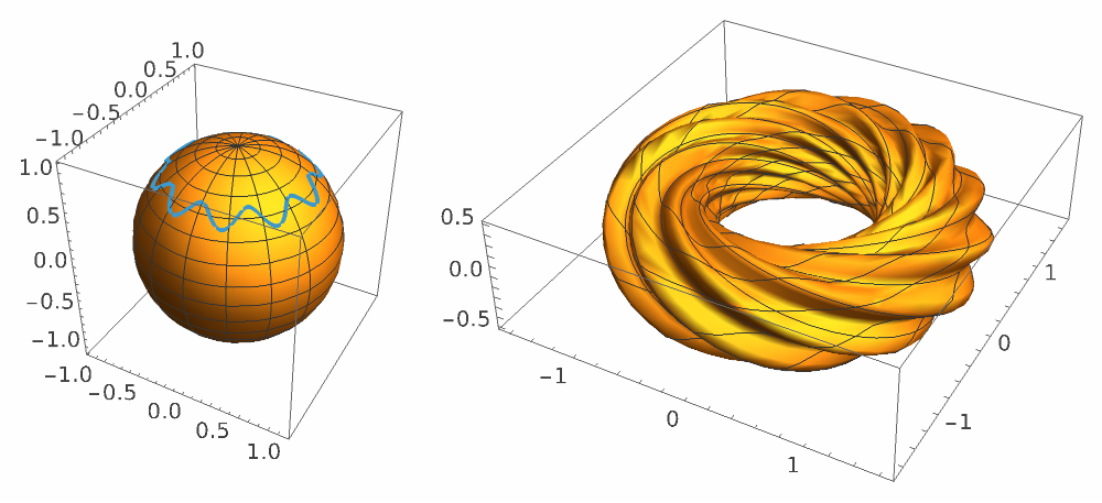
We present an interactive presentation of Hopf tori. The Hopf map π provides the magic behind the generation of tori that projects the three-dimensional sphere onto the two-dimensional sphere . The inverse map maps each point on the two-dimensional sphere into a circle on the three-dimensional sphere. As a consequence, each closed loop on is mapped into a torus embedded in . These tori are visualized through stereographic projection. This is a conformal mapping that preserves angles. You can smoothly deform the closed loop on the to generate all possible conformally distinct two-dimensional tori.
3
S
2
S
-1
π
2
S
3
S
2
S
The following YouTube-short has been the inspiration for this community post: Hopf fibration
The Interactive Torus Generator
The Interactive Torus Generator
In[]:=
Manipulateθ[ϕ_,a_,b_,n_]=a+bCos[nϕ];GraphicsRowShow[{ParametricPlot3D[{Cos[ϕ]Sin[θ],Sin[ϕ]Sin[θ],Cos[θ]},{ϕ,0,2π},{θ,0,π}],ParametricPlot3D[{Cos[ϕ]Sin[θ[ϕ,a,b,n]],Sin[ϕ]Sin[θ[ϕ,a,b,n]],Cos[θ[ϕ,a,b,n]]},{ϕ,0,2π},ImageSize->200]}],ParametricPlot3D,,,{ψ,0,2π},{ϕ,0,2π},PlotRange->All,ImageSize->600,ImageSize->500,a,,"Size",0,π,{{b,0.1,"Amplitude"},0,π/4},{{n,10,"Frequency"},0,20,1}
Cos[ϕ+ψ]Cos[θ[ϕ,a,b,n]/2]
1-Sin[ψ]Sin[θ[ϕ,a,b,n]/2]
Sin[ϕ+ψ]Cos[θ[ϕ,a,b,n]/2]
1-Sin[ψ]Sin[θ[ϕ,a,b,n]/2]
Cos[ψ]Sin[θ[ϕ,a,b,n]/2]
1-Sin[ψ]Sin[θ[ϕ,a,b,n]/2]
π
4
Out[]=


Introduction
Introduction
The Hopf fibration is a mathematical transformation that is used to show that the manifold of the three-dimensional sphere can be understood as a -fiber bundle over the base manifold of a two-dimensional sphere . Therefore, locally the geometry can be understood as a direct product of . The Hopf tori presented in this post give a nice indication how the non-trivial global structure of the fiber bundle looks like. The heart piece of the Hopf fibration is the Hopf map π that maps each point of the onto the two-dimensional sphere . This map surjective. Each point of the has a circle as a pre-image. From this follows that the pre-image of a closed loop must be topologically equivalent to a torus . From complex geometry, we know that each flat torus can be represented by a lattice Take for example the two complex numbers:
3
S
1
S
2
S
2
S
1
S
3
S
2
S
2
S
1
S
1
S
Λ={m+n|m,n∈,,∈}.
ω
1
ω
2
ω
1
ω
2
In[]:=
ω
1
ω
2
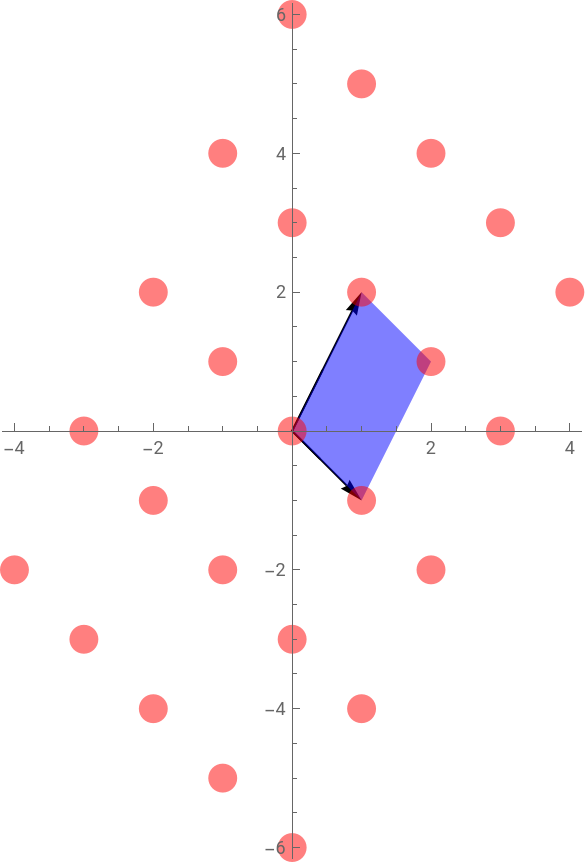
We can visualize parts of the corresponding lattice Λ and its fundamental domain that the torus is associated with. This torus is obtained by identifying opposite sides of the fundamental domain.
In[]:=
Λ=Table[m+n,{m,-2,2},{n,-2,2}];Graphics[{Arrow[{{0,0},ReIm[#]}]&/@{,},Directive[Blue,Opacity[0.5]],Polygon[ReIm[#]&/@{0,,+,}],Directive[Red,PointSize[0.05]],Point[ReIm[#]]&/@Λ},Axes->True]
ω
1
ω
2
ω
1
ω
2
ω
1
ω
1
ω
2
ω
2
Out[]=
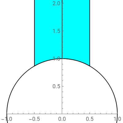
However, not all choices of lattices lead to distinct tori. Some of the lattices can be related by modular transformations. When the modular parameter is introduced, the set of all distinct tori is represented by values of τ that lie inside the fundamental domain of the modular group PSL(2,Z). Any τ outside this light-blue region can be reflected inside this region by a sequence of modular transformations of the form or .
τ=
ω
2
ω
1
1
τ↦τ+1
τ↦-
1
τ
In[]:=
fundamentalDomain=Graphics
Out[]=
It turns that the pre-images of all possible loops generate all possible flat tori. You can use the interactive torus generator to get some intuition how tori of different modular parameters τ can be visualized. It is not possible to visualize the embedded tori isometrically. This would require four spatial dimensions to host the manifold where the tori are embedded to. Instead we show an angle preserving stereographic projection of the tori into our three-dimensional world.
We lay out the following steps to explain the transformations that we used in the interactive torus generator:
It turns that the pre-images of all possible loops generate all possible flat tori. You can use the interactive torus generator to get some intuition how tori of different modular parameters τ can be visualized. It is not possible to visualize the embedded tori isometrically. This would require four spatial dimensions to host the
3
S
We lay out the following steps to explain the transformations that we used in the interactive torus generator:
◼
Loops on
2
S
◼
Hopf coordinates on
3
S
◼
The Hopf map π
◼
The lift of the loop into or the torus embedding
3
S
◼
The stereographic projection of the torus
◼
The complex geometry of the torus
What lies beneath
What lies beneath
Loops on 2S
Loops on
2
S
We simply describe a loop on by a smooth periodic function θ(ϕ). The periodicity θ(ϕ+2π)=θ(ϕ) ensures that the loop is closed. For a sensible solution we also require . Any function θ(ϕ) can be decomposed into Fourier modes . You are invited to customize the interactive torus generator to your needs, implementing as many Fourier components as you wish. However, we decided to use a simpler parameterization for the function . This parameterization only depends on two real parameters and , as well as one integer parameter . These three parameters are sufficient to generate a large variety of tori.
2
S
0≤θ(ϕ)≤π
θ(ϕ)cos(nϕ+)
∞
∑
n0
a
n
ϕ
n
θ(ϕ)a+bcos(nϕ)
a
b
n
θ[ϕ_]:=a+bCos[nϕ];Manipulate

This interactive graphic displays possible loops on . You can use the parameters a, b and n to change the location of the loop, its amplitude and its number of oscillations. For the embedding into we use the standard polar coordinates :
fHowever, instead of the usual parameter ϕ and θ varying freely inside the ranges for the longitude and latitude , the parameter θ is replaced by the function θ(ϕ). Therefore, only one parameter ϕ can vary freely and a one-dimensional loop θ(ϕ) is embedded onto the surface of the two-dimensional sphere .
2
S
2
S
x(θ,ϕ) | sinθcosϕ |
y(θ,ϕ) | sinθsinϕ |
z(θ,ϕ) | cosθ |
0≤ϕ≤2π
0≤θ≤π
2
S
We can verify that all points of the embedding have a unit distance
◼
this is a homogeneous space with constant positive curvature
The induced metric
The induced metric
The Ricci scalar
The Ricci scalar
Next, we compute the Ricci tensor. The implementation of the Ricci tensor is provided at the end of this document. For spaces of constant curvature, the Ricci tensor is just a scaled version of the metric:
The Volume
The Volume
The Hopf Map
The Hopf Map
We can check one more time the consistency of the embedding.
We can introduce new coordinates
Stereographic Projection
Stereographic Projection
This is the parametric plot that is used in our interactive torus generator.
The Geometry of the Torus
The Geometry of the Torus
Similarly, we can grow the torus in the other dimension
Let us start with special cases. When there is no oscillation in θ(ϕ), i.e. θ(ϕ)=a, we have seen that the corresponding torus is a Clifford torus that corresponds to a rectangular fundamental domain.
As soon as you include oscillations into the loop, its length increases, while the enclosed area stays the same. This way, you can create tori with many different modular parameter τ. For me, it was quite surprising to realize how strongly this modular parameter affects the appearance of the torus. Although various sources claim that all these tori are diffeomorphic and only differ in their complex structure. It seems that this complex structure significantly controls the embedding of the torus into the three sphere.
Code
Code
Fundamental Domain
Fundamental Domain
Curvature Computations
Curvature Computations
References
References
1
.P. McCreary, T. J. Murphy and C. Carter, “The Modular Group,” The Mathematica Journal, 9(3), 2005. www.mathematica-journal.com/issue/v9i3.
5
.T. Banchoff. “Geometry of Hopf Mapping and Pinkall’s Tori of Given Conformal Type.” Computers in Algebra. New York, 1990. pp. 57–62.
CITE THIS NOTEBOOK
CITE THIS NOTEBOOK
Hopf fibration: Loops on S² lifted to τ-dependent S³ tori via stereographic projection
by Johannes Martin
Wolfram Community, STAFF PICKS, August 14, 2025
https://community.wolfram.com/groups/-/m/t/3530290
by Johannes Martin
Wolfram Community, STAFF PICKS, August 14, 2025
https://community.wolfram.com/groups/-/m/t/3530290