Numerical Solution of the Falkner-Skan Equation for various Wedge Angles
Authors: Housam Binous and Ahmed Bellagi
Numerical Solution of the Falkner-Skan Equation for various Wedge Angles
Authors: Housam Binous and Ahmed Bellagi
Authors: Housam Binous and Ahmed Bellagi
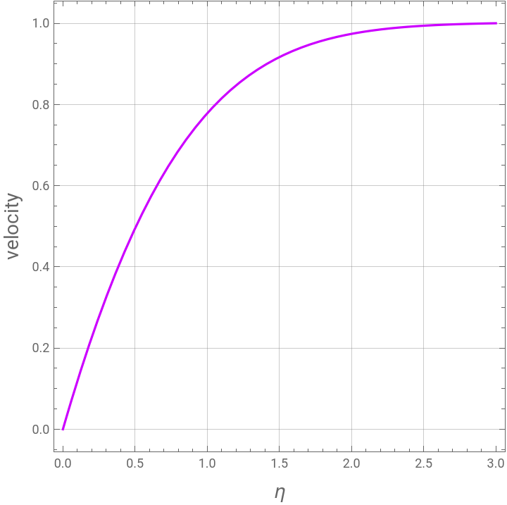
Flow past a wedge is governed by the Falkner - Skan equation . This equation admits only numerical solution, which requires the application of the shooting technique . We plot the velocity for various wedge angles . The result obtained is in agreement with figure 8 - 10 in page 352 of Deen' s book (Analysis of Transport Phenomena, William M . Deen, OUP, 1998) . The well - known Blasius equation appears as a particular case in this study . It represents the flow past a flat plate (parameter β = 0, or a wedge angle equal to zero) . Planar stagnation flow is also treated by the notebook (parameter β = 1 or a wedge angle equal to Pi) .
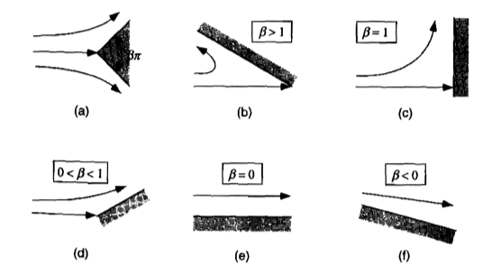
Acknowledgement: The governing equation is taken from Analysis of Transport Phenomena, William M. Deen, OUP, 1998.
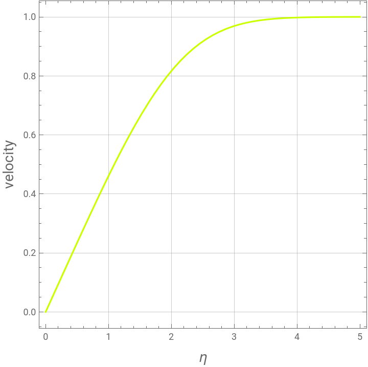
case 1 : β=0. The Blasius equation is recovered.
In[]:=
sol[ξ_]:=NDSolve[{D[f[η],{η,3}]+f[η]f''[η]+β(1-(f'[η])^2)0,f[0]0,f'[0]0,f''[0]ξ},{f[η]},{η,0,5}]
In[]:=
β=0;
In[]:=
DFEnd[ξ_?NumericQ]:=D[f[η]/.sol[ξ],{η,1}]/.η5
In[]:=
SOL1=FindRoot[DFEnd[ξ]1,{ξ,0.5}]
Out[]=
{ξ0.469645}
In[]:=
plt1=Plot[Evaluate[D[f[η]/.sol[ξ/.SOL1],{η,1}]],{η,0,5},PlotStyleHue[1/5],Frame->True,GridLines->Automatic,AspectRatio->1,FrameLabel->{Style["η",14],Style["velocity",14]}]
Out[]=
In[]:=
plt1=Plot[Evaluate[D[f[η]/.sol[ξ/.SOL1],{η,1}]],{η,0,5},PlotStyleHue[1/5],Frame->True,GridLines->Automatic,AspectRatio->1,FrameLabel->{Style["η",14],Style["velocity",14]},PlotLegendsLineLegend[{Hue[1/5],Hue[2/5],Hue[3/5],Hue[4/5],Hue[5/5]},{"β=0","β=0.4","β=-0.199","β=1.0","β=1.6"}]];
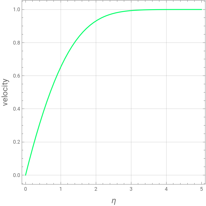
case 2 : β=0.4
In[]:=
β=0.4;
In[]:=
DFEnd[ξ_?NumericQ]:=D[f[η]/.sol[ξ],{η,1}]/.η5
In[]:=
SOL2=FindRoot[DFEnd[ξ]1,{ξ,0.5}]
Out[]=
{ξ0.854422}
In[]:=
plt2=Plot[Evaluate[D[f[η]/.sol[ξ/.SOL2],{η,1}]],{η,0,5},PlotStyleHue[2/5],Frame->True,GridLines->Automatic,AspectRatio->1,FrameLabel->{Style["η",14],Style["velocity",14]}]
Out[]=
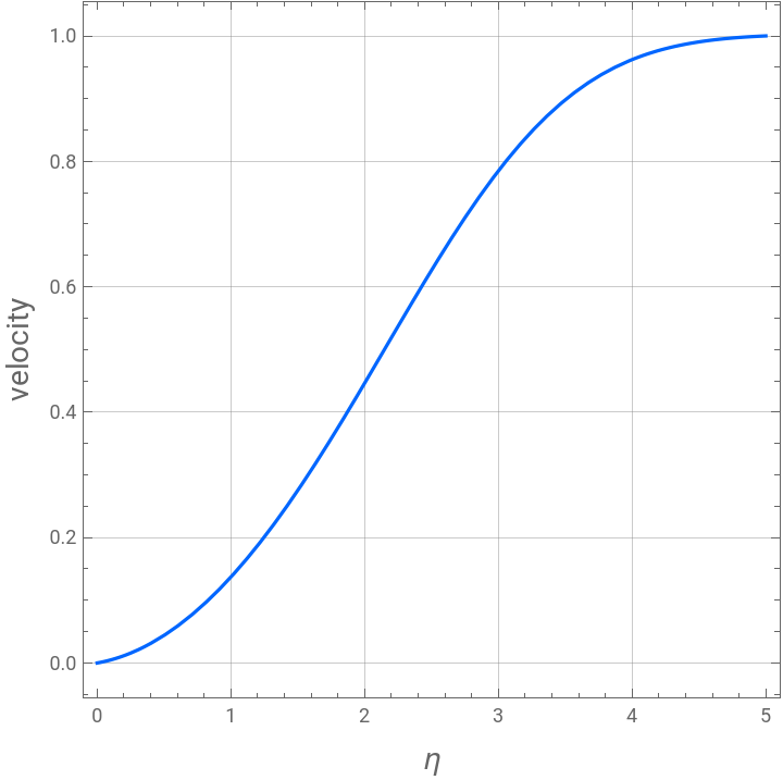
case 3 : β=-0.199
In[]:=
β=-0.199;
In[]:=
sol[ξ_]:=NDSolve[{D[f[η],{η,3}]+f[η]f''[η]+β(1-(f'[η])^2)0,f[0]0,f'[0]0,f''[0]ξ},{f[η]},{η,0,5}]
In[]:=
DFEnd[ξ_?NumericQ]:=D[f[η]/.sol[ξ],{η,1}]/.η5
In[]:=
SOL3=FindRoot[DFEnd[ξ]1,{ξ,0.5}]
Out[]=
{ξ0.0382234}
In[]:=
plt3=Plot[Evaluate[D[f[η]/.sol[ξ/.SOL3],{η,1}]],{η,0,5},PlotStyleHue[3/5],Frame->True,GridLines->Automatic,AspectRatio->1,FrameLabel->{Style["η",14],Style["velocity",14]}]
Out[]=
case 4 : β=1.0
In[]:=
β=1;
In[]:=
sol[ξ_]:=NDSolve[{D[f[η],{η,3}]+f[η]f''[η]+β(1-(f'[η])^2)0,f[0]0,f'[0]0,f''[0]ξ},{f[η]},{η,0,3}]
In[]:=
DFEnd[ξ_?NumericQ]:=D[f[η]/.sol[ξ],{η,1}]/.η3
In[]:=
SOL4=FindRoot[DFEnd[ξ]1,{ξ,0.5}]
Out[]=
{ξ1.23282}
In[]:=
plt4=Plot[Evaluate[D[f[η]/.sol[ξ/.SOL4],{η,1}]],{η,0,3},PlotStyleHue[4/5],Frame->True,GridLines->Automatic,AspectRatio->1,FrameLabel->{Style["η",14],Style["velocity",14]}]
Out[]=
case 5 : β=1.6
In[]:=
β=1.6;
In[]:=
sol[ξ_]:=NDSolve[{D[f[η],{η,3}]+f[η]f''[η]+β(1-(f'[η])^2)0,f[0]0,f'[0]0,f''[0]ξ},{f[η]},{η,0,2.2}]
We obtain the same result as figure 8-10 in page 352 of Deen's book