This is part of live presentation series called Mathematical Games in which we explore a variety of games and puzzles using Wolfram Language. In this episode, we explore some famous equations.
Gardner: The Catenary Curve
Gardner: The Catenary Curve
Gardner mentions many equations, for example the catenary curve.
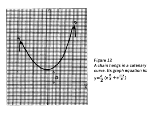
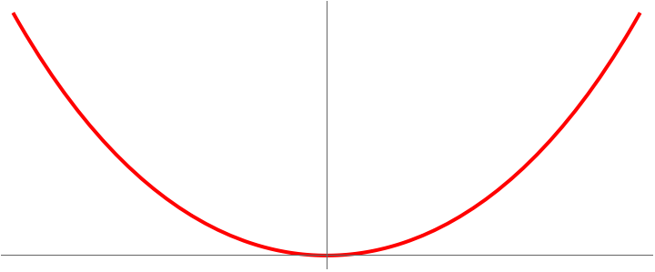
a Cosh[t/a] describes the curve for a hanging chain. 1690: Leibniz, Huygens and Johann Bernoulli. Named by Thomas Jefferson, after the Latin word word for chain: catēna. “I have lately received from Italy a treatise on the equilibrium of arches, by the Abbé Mascheroni. It appears to be a very scientifical work. I have not yet had time to engage in it; but I find that the conclusions of his demonstrations are, that every part of the catenary is in perfect equilibrium.”
In[]:=
Manipulate[Plot[aCosh[t/a],{t,-2,2},AspectRatioAutomatic,PlotStyleRed,TicksNone],{{a,1},.8,4,.1,Appearance->"Labeled"}]
Out[]=


demonstrations.wolfram.com
demonstrations.wolfram.com
Many Demonstrations feature equations
Einstein's Mass–Energy Equivalence
Einstein's Mass–Energy Equivalence
E=m
2
c
Key:
E | Energy(injoules) |
m | Mass(inkilograms) |
c | Speedoflightinvacuum(~3.00×10⁸m/s) |
First published in 1905 by Albert Einstein in his paper *Does the Inertia of a Body Depend Upon Its Energy Content?*, the equation E = mc² revealed that mass and energy are deeply connected. It was later confirmed experimentally, most famously through nuclear reactions in the 1930s and 1940s.
Let's define the speed of light:
c=3.00*
8
10
Example 1: Compute the energy equivalent of 1 kilogram of mass.
m=1;E=m*c^2
Example 2: How much energy is in 0.1 grams of mass?
m=0.1/1000;E=m*c^2
Example 3: How much mass is needed to generate 1 kilowatt-hour of energy?
energyKWh=1*3600*1000;massRequired=energyKWh
2
c
Nuclear reactions convert small amounts of mass to energy.
Euler's Identity
Euler's Identity
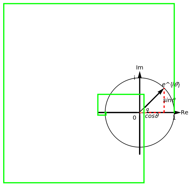
iπ
e
iθ
e
Key:
e | Euler'snumber(~2.718),baseofnaturallogarithms | |
i | Imaginaryunit,definedas√-1 | |
π | Pi,ratioofcircumferencetodiameter(~3.14159) | |
1 | Multiplicativeidentity | |
0 | Additiveidentity |
Introduced by Leonhard Euler in 1748 in his work *Introductio in Analysin Infinitorum*, this equation unites the five most important numbers in mathematics in a single elegant expression. It is often cited as an example of mathematical beauty.
Let's verify it numerically:
In[]:=
N[+1]
Iπ
Out[]=
0.
Gardner wondered how to show it:
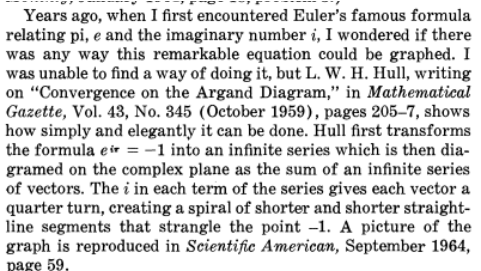
We can do that Taylor series:
In[]:=
Series,{x,0,10}/.x->1
xIPi
E
Out[]=
1+π--++--++-
2
π
2
3
π
6
4
π
24
5
π
120
6
π
720
7
π
5040
8
π
40320
9
π
362880
10
π
3628800
In[]:=
Table[(IPi)^k/Factorial[k],{k,0,10}]
Out[]=
1,π,-,-,,,-,-,,,-
2
π
2
3
π
6
4
π
24
5
π
120
6
π
720
7
π
5040
8
π
40320
9
π
362880
10
π
3628800
In[]:=
N[Total[Table[(IPi)^k/Factorial[k],{k,0,15}]]]
Out[]=
-1.-7.72786×
-7
10
Here’s the spiral:
In[]:=
Graphics[Line[ReIm/@Simplify[Accumulate[Table[(IPi)^k/Factorial[k],{k,0,20}]]]]]
Out[]=
Here’s the spiral on an Argand Diagram:
1+π--++-
2
π
2
3
π
6
4
π
24
5
π
120
6
π
720
Out[]=
Bitcoin: Elliptic Curve Equation
Bitcoin: Elliptic Curve Equation
Here’s a curiously valuable equation:
The curve defines valid points used in Bitcoin's public key cryptography.
This curve is called secp256k1 and is favored for its lack of known backdoors.
Check if a pair of coordinates is on the curve:
In[]:=
p = 2^256 - 2^32 - 977;
x = 55066263022277343669578718895168534326250603453777594175500187360389116729240;
y = 32670510020758816978083085130507043184471273380659243275938904335757337482424;
Mod[y^2 - (x^3 + 7), p]
x = 55066263022277343669578718895168534326250603453777594175500187360389116729240;
y = 32670510020758816978083085130507043184471273380659243275938904335757337482424;
Mod[y^2 - (x^3 + 7), p]
Pythagorean Theorem
Pythagorean Theorem
Key:
This relationship, known since Babylonian times (~1800 BCE) and famously attributed to Pythagoras (~500 BCE), connects the three sides of a right-angled triangle. It laid the groundwork for trigonometry and distance calculations in Euclidean space.
Example 1: If a = 3 and b = 4, find c.
Example 2: If c = 13 and a = 5, find b.
The theorem underlies not only geometry but also distance formulas, vector norms, and digital imaging.
Leavitt’s Law (Cepheid Period–Luminosity Relation)
Leavitt’s Law (Cepheid Period–Luminosity Relation)
Discovered by Henrietta Swan Leavitt in 1908 and refined in 1912.
She put the pulsation period of Cepheid variable stars and their high and low apparent luminosity on a log plot.
Straight lines indicated a direct relation between period and luminosity, a “standard candle.”
It remains a foundation for measuring distances across the universe.
She put the pulsation period of Cepheid variable stars and their high and low apparent luminosity on a log plot.
Straight lines indicated a direct relation between period and luminosity, a “standard candle.”
It remains a foundation for measuring distances across the universe.
Key Equation (absolute magnitude version):
Key Symbols:
m is apparent magnitude
d is distance in parsecs.
d is distance in parsecs.
Thus, Cepheids act as cosmic yardsticks. Measure the period → get M → compare to m → derive distance.
Circles and Spheres
Circles and Spheres
Area of a Circle
Area of a Circle
Known to Babylonian mathematicians, with improved precision by Archimedes (~250 BCE). Basis of π’s early definitions.
Circumference of a Circle
Circumference of a Circle
Linked to π since antiquity. Formal use appears in Euclid’s *Elements* and Archimedean methods.
Volume of a Sphere
Volume of a Sphere
Proved by Archimedes using exhaustion. He famously chose it for his tombstone.
Surface Area of a Sphere
Surface Area of a Sphere
Also due to Archimedes, who discovered it equals the lateral area of the cylinder enclosing the sphere.
Pick's Theorem
Pick's Theorem
Key:
Discovered by Georg Alexander Pick in 1899, this elegant theorem gives an exact formula for the area of any simple lattice polygon using only integer point counts. It's particularly useful in combinatorics, computer graphics, and teaching geometry with dot paper.
Example: A right triangle with vertices at (0,0), (4,0), and (0,3)
The computed area A = 3 + 4 – 1 = 6 matches the usual ½·base·height = 6.
Suppose that a polygon has its corners at the points of a geoboard. (You can drag the corners.) Count the number of boundary points B and interior points I. As long as the polygon does not cross over itself, Pick’s theorem gives the area as A = I + B/2 - 1. In words, the area is one less than the number of interior points plus half the number of border points.
Here’s a function for it:
The Triangle Equation and The Kiss Precise
The Triangle Equation and The Kiss Precise
For the spheres, 0, 1, 1, 1, 3, 4, 7, 13, 21, 37, 64, 109, 189, 325, 559
Euler's Polyhedral Formula
Euler's Polyhedral Formula
Key:
This formula was first published by Leonhard Euler in 1758, showing that for any convex polyhedron—like a cube, tetrahedron, or dodecahedron—the relationship V – E + F = 2 holds true. It’s a gateway to topology and an early whisper of the Euler characteristic.
Example: For a cube: V = 8, E = 12, F = 6
The result is 2, just as Euler promised. For spheres, doughnuts, and stranger shapes, the formula evolves into the Euler characteristic χ.
Quadratic Formula
Quadratic Formula
Key:
The quadratic formula has ancient roots. Babylonian tablets (~2000 BCE) had geometric methods. Al-Khwārizmī (c. 820 CE) provided general algebraic rules. Symbolic forms emerged in 17th-century Europe.
Example: Solve x² + 3x + 2 = 0
Result: x = -1 and x = -2 — two real roots from a positive discriminant.
After that is Cardano’s formula:
Corrected Logarithmic Identity (with Branch Cuts)
Corrected Logarithmic Identity (with Branch Cuts)
Key:
The classical identity log(z_1 z_2) = log(z_1) + log(z_2) was known since the 17th century, particularly after John Napier introduced logarithms in 1614 to simplify multiplication into addition. But in complex analysis, this naive version fails along the branch cut (usually the negative real axis), leading to discontinuities.
This corrected form introduces a floor function to adjust for 2 pi i phase jumps, ensuring the identity holds throughout the complex plane when using the principal branch of the logarithm.
Example: Let z₁ = -1 and z₂ = -1
The classical version fails here: Log[1] = 0, but Log[-1] + Log[-1] = 2 i π — the corrected formula subtracts exactly that.
Some Trigonometry and other Math
Some Trigonometry and other Math
Law of Sines
Law of Sines
Appeared in ancient Greek and Islamic trigonometry, formalized by al-Battani in the 9th century and used in spherical astronomy.
Law of Cosines
Law of Cosines
Used by Euclid (Elements, Book II) in geometric form; modern trigonometric form appears in the 17th century.
Binomial Theorem
Binomial Theorem
Known to Indian and Islamic mathematicians; formalized in Europe by Pascal and Newton. Vital in probability and algebra.
Taylor Series
Taylor Series
Formulated by Brook Taylor in 1715. Expanded by Euler and Lagrange. It expresses smooth functions as infinite sums of derivatives at a point.
This computes a 5th-degree polynomial approximation to sin(x) around x = 0.
Fourier Transform
Fourier Transform
Key:
Example: Transform of a pure sine wave
This gives two spikes at ±3, showing the signal has frequency 3. The Fourier transform maps the sine wave to its frequency spectrum.
Newton’s Difference Quotient (Definition of Derivative)
Newton’s Difference Quotient (Definition of Derivative)
Key:
First formulated by Isaac Newton around 1666 during the Great Plague (a productive quarantine!), this limit-based formula defines the instantaneous rate of change of a function. While Leibniz gave us the familiar notation, Newton's formulation captures the foundational idea of a derivative.
Example: f(x) = x² — compute f'(x)
Use the derivative function:
This returns 2x, confirming the derivative of x² via Newton's method. Every tangent line starts here.
Newton’s Law of Universal Gravitation
Newton’s Law of Universal Gravitation
Key:
Published by Isaac Newton in 1687 in his *Philosophiæ Naturalis Principia Mathematica*, this law described how every mass attracts every other mass with a force proportional to their masses and inversely proportional to the square of the distance between them. It unified earthly physics and celestial motion.
Example: Earth (5.97×10²⁴ kg) and Moon (7.35×10²² kg), distance ≈ 384,400 km
The resulting force is roughly 2×10²⁰ N, which keeps the Moon in orbit—and the tides dancing.
Gaussian (Normal) Distribution
Gaussian (Normal) Distribution
Key:
Named after Carl Friedrich Gauss, who published the distribution in 1809, though it was first described by Abraham de Moivre in 1733. The normal distribution appears in statistics, physics, biology, and anywhere randomness averages out.
Example: Define the standard normal distribution (μ = 0, σ = 1)
The area under the curve equals 1. It’s symmetric about the mean and defines the 68–95–99.7 rule that governs standard deviation zones.
SI Base Quantities and Defining Constants
SI Base Quantities and Defining Constants
As of 2019, the International System of Units (SI) defines its seven base quantities using fixed values of fundamental physical constants. These constants form the core of our modern metrology.
Base Quantities and Corresponding Constants:
These constants are exact by definition. The SI no longer relies on physical artifacts—only on nature’s own bookkeeping.
Deriving the Kilogram via the Kibble Balance (SI Unit of Mass)
Deriving the Kilogram via the Kibble Balance (SI Unit of Mass)
The kilogram is now defined by fixing Planck's constant: h = 6.62607015×10⁻³⁴ J·s. It is realized experimentally through the Kibble (watt) balance, which equates mechanical and electrical power using quantum electrical standards.
Key Equations:
Key Symbols:
Derivation:
Substitute I and V into mgv = IV:
Simplify:
Thus, the kilogram is realized via frequencies, elementary charge, and gravitational/kinematic quantities, all anchored by fixed quantum constants.
Deriving the Second (SI Unit of Time)
Deriving the Second (SI Unit of Time)
Time is defined by fixing the frequency of electromagnetic radiation associated with a hyperfine transition in cesium-133 atoms.
Primary Definition:
That is, one second is the duration of exactly 9,192,631,770 periods of the radiation corresponding to this transition.
Supporting Formulas:
Key Symbols:
Thus, time is measured through periodic motion and wave behavior, and realized with atomic clocks anchored to cesium's hyperfine transition.
Follow-through: calculating one second using the defined frequency of the cesium-133 hyperfine transition.
Given:
Step 1: Compute the period T of one oscillation:
This gives the duration of one cycle of the microwave radiation.
Step 2: Multiply the period by number of cycles (n = 9,192,631,770):
This yields exactly 1 second, by definition. No error, no uncertainty: time itself is now frequency counted.
Conclusion: The second is not measured—it is *counted*, cycle by cycle, using the cesium atom as nature’s metronome.
Defining the Candela (SI Unit of Luminosity)
Defining the Candela (SI Unit of Luminosity)
The candela is the SI base unit of luminous intensity, defined by fixing the luminous efficacy of monochromatic radiation at a frequency of 540×10¹² Hz (green light).
Key Equations:
Key Symbols:
Derivation: start from photon energy at f = 540 THz:
Compute power from photon stream:
Determine radiance per steradian and area, then luminous intensity:
Thus, 1 candela is the luminous intensity of a source emitting monochromatic radiation of frequency 540 THz and radiant intensity 1/683 W per steradian.
Defining the Kelvin (SI Unit of Temperature)
Defining the Kelvin (SI Unit of Temperature)
Since 2019, the kelvin is defined by fixing the Boltzmann constant to exactly 1.380649×10⁻²³ J/K. Temperature is thus a measure of average energy per degree of freedom.
Key Equations:
Key Symbols:
Derivation: Start with particle energy in an ideal gas:
Solve for T:
Thus, 1 kelvin corresponds to an average energy of 1.380649×10⁻²³ joules per particle per degree of freedom.
All of physics can now easily be derived
All of physics can now easily be derived
Defined and derived units
Defined and derived units
Defined
Defined
Derived
Derived
Newton's Second Law of Motion
Newton's Second Law of Motion
Key:
Formulated by Sir Isaac Newton in 1687 in his *Philosophiæ Naturalis Principia Mathematica*, this equation describes how an object’s motion changes when a force is applied. It remains central to classical mechanics.
Example 1: Find the force needed to accelerate a 10 kg object at 2 m/s².
Example 2: Given a force of 50 N and a mass of 5 kg, find the acceleration.
Newton’s Second Law explains motion from rockets to roller coasters. It tells us why kicking a bowling ball hurts more than kicking a ping pong ball.
Motion Quantities: Kinematics and Dynamics
Motion Quantities: Kinematics and Dynamics
Defines location in space over time.
Rate of change of position. Units: m/s
Change of velocity over time. Units: m/s²
Rate of change of acceleration. Units: m/s³
Fourth derivative of position. Rare in physics; units: m/s⁴
Mass in motion. Units: kg·m/s
Time derivative of force. Units: N/s
Change in momentum. Units: N·s = kg·m/s
Key:
Fundamental Theorem of Calculus
Fundamental Theorem of Calculus
Key:
This theorem was formalized in the late 1600s by Newton and Leibniz, and it bridges differential and integral calculus. Part 1 says accumulation defines a function whose derivative is the original; Part 2 lets you compute that accumulation via antiderivatives.
Example: f(x) = 3x² ⇒ F(x) = x³
This returns 7, the same as x³ evaluated from 1 to 2. Derivatives undo integrals; integrals capture net change.
Bayes’ Rule
Bayes’ Rule
Key:
Proposed by Thomas Bayes in the 18th century and popularized by Laplace, Bayes’ Rule gives a principled way to update probabilities in light of new data. It’s foundational in statistics, machine learning, and decision theory.
Example: Disease testing (1% prevalence, 99% sensitivity/specificity)
Even with a positive test, the chance you're actually sick is only about 50%—Bayes corrects our intuitions about rare events.
Fermat's Little Theorem
Fermat's Little Theorem
Key:
This theorem, stated by Pierre de Fermat in 1640, is a fundamental result in number theory and modular arithmetic. It’s used in cryptography, primality testing, and proofs involving finite fields.
Example: a = 3, p = 7
Output: 1, since 3⁶ = 729 and 729 mod 7 = 1
Shannon Entropy
Shannon Entropy
Key:
Introduced by Claude Shannon in 1948, this formula measures the average uncertainty of a random variable. Uniform distributions have higher entropy; predictable ones have less.
Example: A fair 4-sided die
This evaluates to 2 bits, the max for 4 outcomes. Bias the probabilities, and entropy falls.
Black–Scholes Equation
Black–Scholes Equation
Key:
Developed by Fischer Black and Myron Scholes in 1973, this equation revolutionized financial markets by providing a replicable strategy to hedge risk and price European-style options under certain assumptions.
Example: Define the Black-Scholes PDE in symbolic form
The exact solution (Black–Scholes formula) uses cumulative normal distributions and assumes no arbitrage, constant volatility, and frictionless markets.
D’Alembert’s Wave Equation
D’Alembert’s Wave Equation
Key:
First derived by Jean d’Alembert in 1747 for vibrating strings, this equation describes any wave propagating through a linear medium. It's symmetric in space and time, and its solutions travel without distortion.
Example: General solution as a pair of traveling waves
Any initial waveform splits into left- and right-traveling waves at speed c. The superposition creates the full solution.
First derived by Jean d'Alembert in 1747 for vibrating strings, this equation describes any wave propagating through a linear medium. It's symmetric in space and time, and its solutions travel without distortion.
This equation models vibrating strings and other ideal wave media. The general solution is the sum of left- and right-traveling waves.
Define constants and wave components:
In[]:=
c = 1;
f[z_] := Sin[z]; g[z_] := Cos[z];
u[x_, t_] := f[x - c t] + g[x + c t];
Plot3D[u[x, t], {x, 0, 10}, {t, 0, 10}, AxesLabel -> {"x", "t", "u"}, PlotRange -> All]
f[z_] := Sin[z]; g[z_] := Cos[z];
u[x_, t_] := f[x - c t] + g[x + c t];
Plot3D[u[x, t], {x, 0, 10}, {t, 0, 10}, AxesLabel -> {"x", "t", "u"}, PlotRange -> All]
Dirac's Equation
Dirac's Equation
Key:
Proposed in 1928 by Paul Dirac, this equation unified quantum mechanics with special relativity and provided the first theoretical prediction of antimatter. By introducing spinor fields and gamma matrices, it naturally incorporates spin-½ particles and ensures Lorentz invariance. Dirac’s equation explains the fine structure of hydrogen and laid the foundation for quantum field theory.
Example: Free particle solution (not computed here, but symbolic)
Where u is a constant spinor and p·x is the Minkowski inner product.
Cauchy’s Residue Theorem
Cauchy’s Residue Theorem
Key:
Cauchy's Residue Theorem (c. 1825) reduces contour integrals to a sum of local residues. A foundational tool in evaluating real and complex integrals.
Example: Integrate 1 / (z² + 1) around the unit circle
The residues cancel: the net integral is zero. Symmetry in action.
Maxwell's Equations
Maxwell's Equations
Key:
Published in their final form by James Clerk Maxwell in 1865, these equations unified electricity and magnetism into a single framework: classical electromagnetism. They predicted electromagnetic waves—light—as a self-propagating disturbance in electric and magnetic fields.
Example: In empty space (ρ = 0, J = 0), combine equations to derive the wave equation for E:
Einstein Field Equations
Einstein Field Equations
Key:
Einstein published these equations in 1915, completing general relativity. They describe how matter and energy determine the curvature of spacetime. From black holes to the expanding universe, the EFE rules them all.
Example: Schwarzschild metric for vacuum solution
In[]:=
g = DiagonalMatrix[{-(1 - 2 G M/r), 1/(1 - 2 G M/r), r^2, r^2 Sin[θ]^2}]
This metric solves the vacuum EFE when Tμν = 0
Euler–Lagrange Equation
Euler–Lagrange Equation
Key:
Developed in the 18th century by Euler and Lagrange, this equation replaces Newton's laws with a variational principle. It's the core of classical mechanics, field theory, and modern physics.
Define the Lagrangian for a free particle
In[]:=
L[q_, qdot_] := (1/2) m qdot^2
Euler–Lagrange equation components
In[]:=
D[L[q[t], q'[t]], q'[t]] // D[#, t] & - D[L[q[t], q'[t]], q[t]]
This simplifies to m q''[t] == 0 — constant velocity
Planck’s Equation for Photon Energy
Planck’s Equation for Photon Energy
E = h ν
Key:
First introduced by Max Planck in 1900 to explain blackbody radiation, this equation established the foundation of quantum theory. It implies that light and other electromagnetic waves are quantized—carried by discrete packets of energy called photons.
In[]:=
h = 6.626*10^-34;
ν = 4.3*10^14;
EE = h*ν
ν = 4.3*10^14;
EE = h*ν
In[]:=
eV = 1.602*10^-19;
ν = eV/h
ν = eV/h
Planck’s Law of Blackbody Radiation
Planck’s Law of Blackbody Radiation
This equation gives the spectral radiance of a blackbody at frequency ν and temperature T. It resolved the ultraviolet catastrophe by introducing quantized energy packets.
Key:
Example: Plot Planck’s radiation law at 3000 K and 6000 K.
Higher temperature shifts the peak to higher frequencies, avoiding the classical ultraviolet divergence.
Lotka–Volterra Predator–Prey Model
Lotka–Volterra Predator–Prey Model
These coupled nonlinear equations model the interaction between a prey population (x) and a predator population (y).
Key:
Example: Define parameters and simulate dynamics numerically.
The predator and prey populations oscillate out of phase, forming closed loops in phase space. The model is idealized but captures key ecological dynamics.
Navarro Tariff Equation
Navarro Tariff Equation
This equation was presented in public materials from the USTR to support reciprocal tariffs. It calculates the tariff change Δτ_i needed to eliminate the trade deficit with country i.
Key:
The formula assumes a full pass-through of tariffs to exporter prices (i.e., φ ≈ 1), and elasticity ε such that ε·φ ≈ 1,
simplifying the equation to (xᵢ - mᵢ)/mᵢ. Instead of targeted tariffs, trade deficits were divided by imports. Also, the tariffs were split by internet domains, which is why territories and uninhabited regions received tariffs.
simplifying the equation to (xᵢ - mᵢ)/mᵢ. Instead of targeted tariffs, trade deficits were divided by imports. Also, the tariffs were split by internet domains, which is why territories and uninhabited regions received tariffs.
The formula cites a 2011 book by Navarro, which in turn cites the fictional trade expert Ron Vara (an anagram of Navarro).
Example: $200B trade deficit, $500B imports, ε·φ assumed 1
Result: 40% tariff. But this assumes exporters reduce their prices by the full tariff amount, and U.S. consumers are unaffected—an assumption not supported by trade data.
Heisenberg’s Uncertainty Principle
Heisenberg’s Uncertainty Principle
This equation places a fundamental limit on the simultaneous precision of position and momentum measurements. The more precisely one is known, the less precise the other can be.
Key:
Example 1: If δx = 1 nm, what is the minimum δp?
This principle is not due to measurement error, but to the wave-like nature of matter itself. It marks a fundamental departure from classical determinism.
Example: Rauch & Werner, Neutron Interferometry (Oxford, 2000)
Neutrons are passed through an interferometer slit or narrow guide
Their spatial distribution is measured on a detector screen
Their momentum spread is known from beamline energy calibration
Neutrons are passed through an interferometer slit or narrow guide
Their spatial distribution is measured on a detector screen
Their momentum spread is known from beamline energy calibration
Sparse Ruler Excess Equation
Sparse Ruler Excess Equation
This equation gives the excess E(n) of a sparse ruler of length n. It measures how many more marks (m) are used than the theoretical minimum necessary to measure all integer distances from 1 to n.
Key:
History:
History:
Sparse rulers were first explored in the 1940s in relation to radio antenna design. The excess equation emerged from later combinatorial research, with this bound appearing in computational work around 2020 as part of sparse ruler optimization and OEIS sequence A326499.
Example: A ruler of length 51 with 13 marks
Result: E = 1, meaning this ruler uses one more mark than the minimum required by the theoretical bound.
Mandelbrot and Julia Sets
Mandelbrot and Julia Sets
This recursive equation defines both the Mandelbrot and Julia sets. The iteration zₙ₊₁ = zₙ² + c forms the foundation of complex dynamical systems.
Key:
Mandelbrot Set:
Mandelbrot Set:
Discovered by Benoit Mandelbrot in 1980 using computer graphics. It is the set of all c ∈ ℂ for which the sequence zₙ₊₁ = zₙ² + c with z₀ = 0 does not diverge. The boundary of this set displays infinite complexity and self-similarity.
Julia Sets:
Julia Sets:
First analyzed by Gaston Julia and Pierre Fatou between 1918 and 1920. For a fixed c, the Julia set is the boundary between initial values z₀ that escape to infinity and those that remain bounded under iteration.
Historical:
Historical:
Gaston Julia (1893–1978) and Pierre Fatou (1878–1929) studied these mappings rigorously in the 1910s. Mandelbrot revived interest in 1980 by visualizing the set now bearing his name, giving birth to fractal geometry.
Hamilton's Equations
Hamilton's Equations
Key:
Hamilton’s framework describes motion as a flow through phase space, where energy gradients steer the evolution.
Example: Simple Harmonic Oscillator
In[]:=
H[q_, p_] := p^2/2 + (k/2)*q^2
In[]:=
qdot = D[H[q, p], p]
In[]:=
pdot = -D[H[q, p], q]
These yield q̇ = p and ṗ = –kq. A full loop in phase space—no energy lost.
Doppler Shift and Redshift of Galaxies
Doppler Shift and Redshift of Galaxies
The Doppler effect describes how the observed wavelength of light shifts when a source moves relative to an observer. For galaxies, redshift reveals recessional velocity and distance.
Key Equations:
Key Symbols:
Example: A galaxy’s spectral line (λ_emit = 500 nm) is observed at λ_obs = 550 nm.
In[]:=
z = (550 - 500)/500
→ z = 0.1 ⇒ v ≈ 0.1c ≈ 30,000 km/s
In[]:=
H0 = Quantity[70, "Kilometers"/"Seconds"/"Megaparsecs"];
In[]:=
d = N[v/H0] // UnitConvert[#, "Megaparsecs"] &
→ d ≈ 428.3 Mpc using H₀ = 70 km/s/Mpc
Thus, redshift tells us both how fast a galaxy is receding and how far away it lies in an expanding universe.
Euler–Lagrange Equation
Euler–Lagrange Equation
This equation arises from the principle of stationary action. It determines the path a system takes by minimizing the action integral.
Key:
History:
History:
Derived by Euler (1755) and extended by Lagrange (1760), this equation governs all classical mechanics derived from variational principles.
(* Define q as a time function *)
In[]:=
L = 1/2 m q'[t]^2 - 1/2 k q[t]^2;
In[]:=
D[D[L, q'[t]], t] - D[L, q[t]] // Simplify
Riemann Hypothesis: Zeta Function Zeros
Riemann Hypothesis: Zeta Function Zeros
Unsolved
ζ(s) = 0 ⟹ Re(s) = 1/2
Key:
History:
Proposed by Bernhard Riemann in 1859, this unproven conjecture underpins the distribution of prime numbers and is one of the seven Clay Millennium Problems.
Plot zeta(s) along the critical line
In[]:=
ListLinePlot[Table[ReIm[Zeta[1/2 + I t]], {t, 0.1, 50, 0.1}],PlotRange -> All, AxesLabel -> {"Re", "Im"}, PlotStyle -> Blue]
Navier–Stokes Equation (Incompressible Form)
Navier–Stokes Equation (Incompressible Form)
Unsolved: Do smooth solutions always exist in 3D?
Key:
First developed by Claude-Louis Navier in 1822 and refined by George Gabriel Stokes in 1845, this equation governs the motion of viscous fluids. Despite its wide use—from weather models to inkjets—the general solution remains elusive in three dimensions.
Example: Define a simple 2D velocity field and compute the advective term
This simple rotation field is divergence-free, matching the incompressible assumption. The full Navier–Stokes analysis adds time-dependence, pressure, viscosity, and more swirling wonder.
Schrödinger's Equation and the Wheeler–DeWitt equation
Schrödinger's Equation and the Wheeler–DeWitt equation
Unsolved: is the Wheeler–DeWitt equation valid?
Key:
Introduced by Erwin Schrödinger in 1926, this equation is the foundation of non-relativistic quantum mechanics. It governs how quantum states evolve in time and underlies all wave-based quantum predictions. The Wheeler–DeWitt equation, by contrast, attempts to apply quantum mechanics to the entire universe — and controversially, contains no explicit time.
Example: This defines the Hamiltonian operator as a function acting on ψ(x)
In practice, solving Schrödinger's equation means finding how ψ(x,t) behaves for different potentials, like wells, barriers, or harmonic oscillators.
CITE THIS NOTEBOOK
CITE THIS NOTEBOOK
Mathematical Games: Famous Equations
by Ed Pegg
Wolfram Community, STAFF PICKS, April 24, 2025
https://community.wolfram.com/groups/-/m/t/3449605
by Ed Pegg
Wolfram Community, STAFF PICKS, April 24, 2025
https://community.wolfram.com/groups/-/m/t/3449605