The project targets to define product and sum operators represented by the graphs or the hypergraphs. These are used to construct the operator algebra with it. To define the sum and product operations, a suitable matrix representation for the graphs needs to be determined. These operations are later used to construct (anti-) commutators of matrices that describe operators in quantum mechanics and their graphs are studied.
In the scope of the project an ‘edge exclusion hypothesis’ regarding graphs of anti-commuting matrices arose, which claims to find a link between the graphs and their compliments and the anti-commuting properties of matrices.
During the project, multiplication and addition of graphs was represented by the operations on adjacent matrices, which was achieved both using regular definitions and rules for rewrite systems. The latter motivated a new definition of graph - a unigraph, which allowed to achieve confluence for the product operation.
As the rewrite system of the matrix product was only achieved for the adjacency matrices, it would be interesting to see whether/how the same can be implemented for the weighted adjacency matrices. Further, it would be interesting to see, how the ‘edge exclusion hypothesis’ can be generalized for the arbitrary odd dimensional matrices.
Section 1: Sum and Product operations
Section 1: Sum and Product operations
In the following we will use the weighted graphs, unless stated otherwise. A weighted graph is a graph in which each branch is given a numerical weight. A weighted graph is therefore a special type of labeled graph in which the labels are numbers .
To represent graphs in matrix form, (weighted) adjacency matrices will be used. An adjacency matrix is a square matrix used to represent a finite graph. The elements of the matrix indicate whether pairs of vertices are adjacent or not in the graph. If we consider a matrix B to represent an arbitrary finite graph, the elements of such matrix will be:
To represent graphs in matrix form, (weighted) adjacency matrices will be used. An adjacency matrix is a square matrix used to represent a finite graph. The elements of the matrix indicate whether pairs of vertices are adjacent or not in the graph. If we consider a matrix B to represent an arbitrary finite graph, the elements of such matrix will be:
1
.a non-zero element that indicates an edge from i to j
B
ij
2
.a zero element , if there is no edge from i to j
B
ij
1.1 Sum Rule
1.1 Sum Rule
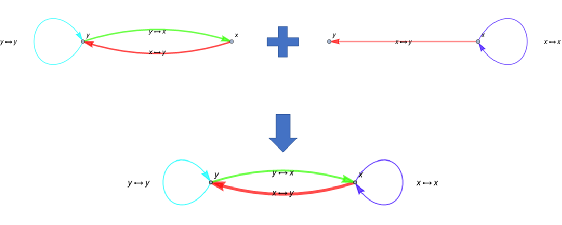
In the following we will represent the sum rule on an example of two matrices A = and B = and the resulting matrix C = A + B = as graphs. As all three graphs possess the same vertices, the highlighted edges of the same color represent the elements on the same positions for each matrix. The weights of the edges are shown through their thickness.
0 | 2 |
2 | 1 |
1 | 1 |
0 | 0 |
1 | 3 |
2 | 1 |
The graph corresponding to the matrix A looks as follows:
Out[]//MatrixForm=
0 | 2 |
2 | 1 |
Out[]=
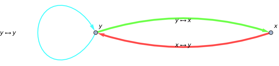
And the graph corresponding to the matrix B is:
Out[]//MatrixForm=
1 | 1 |
0 | 0 |
Out[]=
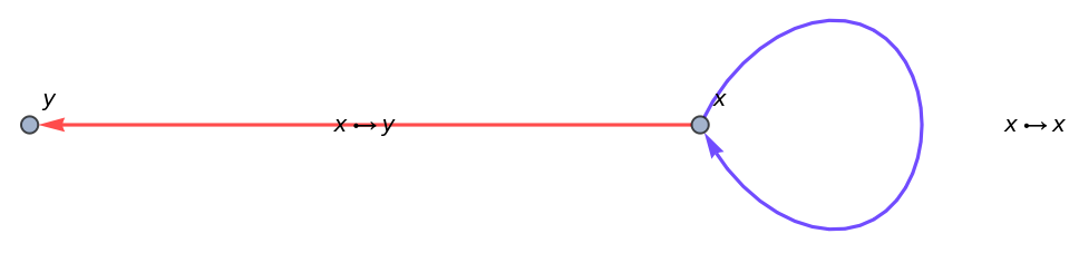
Their sum C is then given as:
Out[]//MatrixForm=
1 | 3 |
2 | 1 |
Out[]=

Where the last graph is obtained by combining the highlighted contributions of the first two graphs. Notably, the thickness of the overlapping edges between the graphs A and B contributed to the increased thickness of the final graph C.To summarize:
1.2 Product Rule
1.2 Product Rule
Similarly to the previous section, we will represent the product of two matrices A = and B = and the resulting matrix C = AB = as graphs. Geometrically one can view graph multiplication as follows:Suppose A is the adjacency matrix of graph (highlighted in green) and B the adjacency matrix of graph (highlighted in blue), where we consider both and to have the same vertices 1,...,n. Then, is the number of ways to get from i to j by going first along an edge of and then along an edge of . We are going to illustrate this below.Starting with the graph representation of the matrix A:
0 | 2 |
2 | 1 |
1 | 1 |
0 | 0 |
0 | 0 |
2 | 2 |
G
1
G
2
G
1
G
2
(AB)
ij
G
1
G
2
Out[]//MatrixForm=
0 | 2 |
2 | 1 |
Out[]=
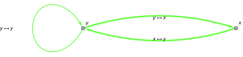
And the graph representation of the matrix B:
In[]:=
bmat={{1,1},{∞,∞}};bthick={1,1};bcolor={0.7,0.7};bgraph=WeightedAdjacencyGraph[{x,y},bmat,VertexLabels->Automatic,EdgeLabels->All,EdgeStyle->Thread[{x->y,x->x}->Thread@{(Hue[#]&/@bcolor),(Thickness[#/300]&/@bthick)}],DirectedEdges->True,EdgeStyle->Arrowheads[Medium]];WeightedAdjacencyMatrix[bgraph]//MatrixFormbgraph
Out[]//MatrixForm=
1 | 1 |
0 | 0 |
Out[]=
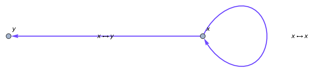
First, we compute the matrix AB:
Out[]//MatrixForm=
0 | 0 |
2 | 2 |
Out[]=
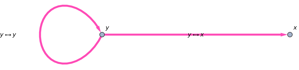
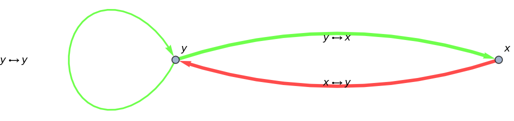
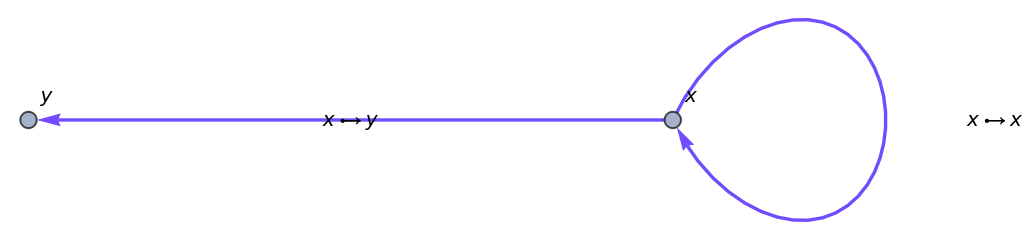
The geometric interpretation for each one of four elements of C = AB.
Starting from: How many ways are there to get from x in to x in ? (The contributing paths are colored in red)
Starting from
(AB)
11
G
1
G
2
G1:
Out[]=
G2:
Out[]=
Complete path:
In[]:=
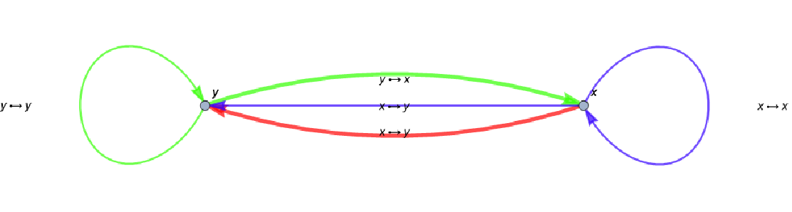
As we can see, there is no way of coming to back to x in the graph , thus we get = 0.
: How many ways are there to get from x in to y in ?
G
2
(AB)
11
(AB)
12
G
1
G
2
G1:
G2:
Complete path:
G1:
G2:
Complete path:
G1:
G2:
Complete path:
1.3 Connection to rewrite systems
1.3 Connection to rewrite systems
1.3.1 Directed Multigraphs
1.3.1 Directed Multigraphs
In order to keep track of the edges of the given graph pair, we promoted both to the hypergraphs. In doing so, we bind all edges of the first graph A to a point 1 and all the edges of the second graph B we will bind to a point 2. Similarly, the third graph that will result from the manipulations on A and B will be bounded to a point 3. Thus, we can always distinct the three graphs. To implement the graph multiplication using the rewrite system, two rules are defined:
◼
Take an edge from the first graph A and an edge from the second graph B, turn them into an edge in the third graph. Reintroduce the used edges of graphs A, B.
◼
Delete all duplicate edges of the third graph C
Even though, the obtained result does not reach confluence, it still manages to provide the graph multiplication after two generations.
1.3.2 Unigraph
1.3.2 Unigraph
Compared to multigraph, which consists of multiset of pairs, the unigraph consists of sets of pairs. Thus, the problem of confluence is resolved by definition of the set. The elements of matrix representing a unigraph may only contain zeros and ones with the additional rule: 1 + 1 = 1. Application of the unigraph notion to the graph product of A and B results in a graph represented by binary matrix C. While this approach does not preserve weights, the results is confluent.
Section 2: Commutator and Anticommutator
Section 2: Commutator and Anticommutator
Using the definitions of graph product and graph sum from the previous section, we can now construct the (anti-)commuting matrices and analyze them.
2.1 Commutator
2.1 Commutator
In this section we search for graphs that represent matrices A,B satisfying the following commutation relation:
[A,B] = AB - BA = 0
To simplify the calculations, only symmetric matrices will be considered at the moment. The algorithm of finding the graphs of interest goes as follows:
[A,B] = AB - BA = 0
To simplify the calculations, only symmetric matrices will be considered at the moment. The algorithm of finding the graphs of interest goes as follows:
◼
Pick a random symmetric matrix A
◼
Find its eigenvectors
◼
From the eigenvectors construct another matrix B with random eigenvalues
◼
Visualise the corresponding graphs
The weights of the edges are represented by their opacity, positive weights are colored green and the negative ones are colored purple.
The random commuting matrices and their graphs are given as:
The random commuting matrices and their graphs are given as:
Where the maximum difference between two elements is of order of machine precision:
An observation can be made at this point: Analogically to how multiple bosons are able to possess the same energy level, so do the edges that can unite the same two vertices in both commuting matrices. This will contrast to how the anti-commuting graphs behave.
2.2 Anticommutator
2.2 Anticommutator
In this section we search for graphs that represent matrices A, B satisfying the following anti-commutation relation:
{A,B} = AB + BA = 0
{A,B} = AB + BA = 0
2.2.1 Small matrices
2.2.1 Small matrices
And the corresponding anticommutator:
And the corresponding anti-commutator:
Any graph from above is the complement of the other two (we treat the real and imaginary weights differently). This motivates a hypothesis that two symmetric (self-adjoint) graphs with excluded edges anti-commute, we will call this an ‘edge exclusion hypothesis’.
Conversely, starting from two vertices we can derive Pauli matrices by drawing pairs of graphs with excluded edges. We will develop a more precise formulation of the commuting matrices below. Additionally, using the resulting graphs and the graph corresponding to the unitary matrix, and the product/sum rules from above, we can construct any graph between two vertices.
Conversely, starting from two vertices we can derive Pauli matrices by drawing pairs of graphs with excluded edges. We will develop a more precise formulation of the commuting matrices below. Additionally, using the resulting graphs and the graph corresponding to the unitary matrix, and the product/sum rules from above, we can construct any graph between two vertices.
Once again, we see that the anti-commuting graphs seem to agree with the ‘edge exclusion hypothesis’.
2.2.2 Generalization for an arbitrary dimension
2.2.2 Generalization for an arbitrary dimension
And the corresponding matrices indeed commute up to machine precision:
2.2.3 Edge exclusion hypothesis
2.2.3 Edge exclusion hypothesis
Finally, we count ones and divide by the matrix dimension. For the example above we get:
Doing the same operation for the Dirac matrices and higher dimensional matrices, we obtain a plot:
As the number of intersections per dimension does not grow for the bigger matrices, we may indeed conclude, that there is a pattern present. Thus, the plot is in the agreement with an assumption of the ‘edge exclusion hypothesis’ in higher-order gamma matrices.
Concluding remarks
Concluding remarks
The algebra of graph operators has proven to be an interesting topic with a large number of undiscovered properties. In scope of this project, we have shown the multiple ways to define a graph product, especially the definition with regards to unigraph seems to have a lot of potential.
Using the operations of addition and multiplication, we have found a way to construct (anti-)commuting graphs. In case of the anti-commutation, a farther insight has been provided - two graphs that have excluded edges anti-commute, this has been called an ‘edge exclusion hypothesis’, as it is similar to the Pauli exclusion principle for the fermions.
In the future it would be meaningful to investigate the project further for the following points still need to be addressed:
◼
Isomorphism of local subgraphs of the the graph product multiway system
◼
Generalization of the graph product using the rewrite system to the weighted graphs, retaining the confluence
◼
Search for topological properties in (anti-)commuting graphs
◼
Proof and further generalization of the edge exclusion hypothesis
◼
Discussion of odd-dimensional (anti-)commuting graphs
Keywords
Keywords
◼
Adjacency Matrix
◼
Graph Product
◼
Unigraph
◼
Commuting Graphs
◼
Anti-commuting Graphs
◼
Edge exclusion hypothesis
Acknowledgment
Acknowledgment
I would like to sincerely thank my mentors, Xerxes Arsiwalla and Jon Lederman, for their invaluable input and support. Also, I can’t over-appreciate the help of Tali Beynon, who explained a lot of graph theory and wrote a function for the discussion of unigraphs.
My gratitude goes to Steven Wolfram, who helped define my project and made valuable comments during the Mid-Course corrections.
My gratitude goes to Steven Wolfram, who helped define my project and made valuable comments during the Mid-Course corrections.
References
References
◼
Adjacency matrix: https://en.wikipedia.org/wiki/Adjacency_matrix
◼
Multisets: https://quivergeometry.net/multisets/
◼
Higher-order Gamma Matrices: https://en.wikipedia.org/wiki/Higher-dimensional_gamma _matrices