ABSTRACT: To describe the charge-polarization coupling in the nanostructure formed by a thin HfxZr1-xO2 film with a single-layer graphene as a top electrode, we develop the “effective” Landau-Ginzburg-Devonshire model. The free energy is expanded in the powers of two order parameters, polarization P and anti-polarization A. The resulting free energy is minimized analytically using Mathematica(R) symbolic calculus. The dynamic dependences of P and A on the electric field are obtained by solving Landau-Khalatnikov equations with the help of NDSolve function. Our approach is based on the parametrization of the Landau expansion coefficients for the polar (FE) and antipolar (AFE) orderings in thin Hf1-xZrxO2 films from a limited number of polarization-field curves and hysteresis loops. The Landau expansion coefficients are nonlinearly dependent on the film thickness h and Zr/[Hf+Zr] ratio x, in contrast to h-independent and linearly x-dependent expansion coefficients of a classical Landau energy. We explain the dependence of the Landau expansion coefficients by the strong nonmonotonic dependence of the Hf1-xZrxO2 film polar properties on the film thickness, grain size and surface energy. The proposed Landau free energy with five “effective” expansion coefficients, which are interpolation functions of x and h, describes the continuous transformation of polarization dependences on applied electric field and hysteresis loop shapes induced by the changes of x and h in the range 0 < x < 1 and 5 nm < h < 35 nm. Using the effective free energy, we demonstrated that the polarization of Hf1-xZrxO2 film influences strongly on the graphene conductivity, and the full correlation between the distribution of polarization and charge carriers in graphene is revealed. In accordance with our modeling, the polarization of the (5 - 25) nm thick Hf1-xZrxO2 films, which are in the ferroelectric-like or antiferroelectric-like states for the chemical compositions 0.35<x< 0.95, determine the concentration of carriers in graphene and can control its field dependence. CITATION (original article): Anna N. Morozovska et al. (2023), “Effective Landau-type model of a HfxZr1−xO2-graphene nanostructure”, Phys. Rev. Applied 20(05):054007, https://doi.org/10.1103/PhysRevApplied.20.054007
Definitions
Definitions
PAdiagram: function to find the absolute minimum of the free energy with respect to polarization, P, and anti-polarization, A, order parameters (Kittel-like model)
PAdiagram: function to find the absolute minimum of the free energy with respect to polarization, P, and anti-polarization, A, order parameters (Kittel-like model)
Loops: functions for the calculations of polarization P and antipolarization A hysteresis loops
Loops: functions for the calculations of polarization P and antipolarization A hysteresis loops
Figures
Figures
Phase-Diagrams: (ap, aa)-space (Figure 2)
Phase-Diagrams: , )-space (Figure 2)
(
a
p
a
a
The phase transitions between different phases are possible when their corresponding free energy values are equal to each other. The transition “curves” could be found numerically by finding the minimal value from the List of the energy values, calculated analytically. These curves could be combined together to visualize the phase diagram
Diagrams representing the different phases of the considered system are plotted with the help of ContourPlot
In[]:=
AlphaP[x_]:=x;AlphaA[y_]:=y;
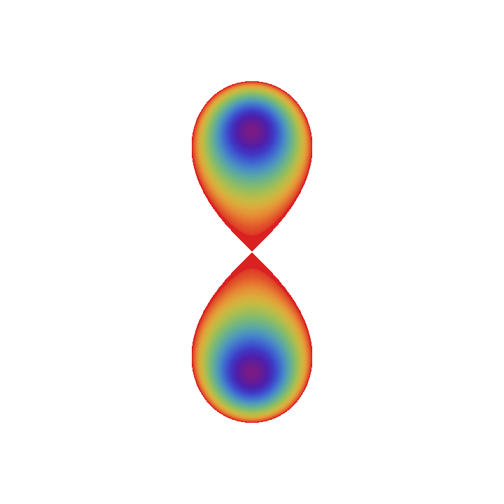
Typical energy profiles in the order parameters space (coordinates (P, A))
In[]:=
beta=1;eta=0.99;limit=2.0;ContourPlot[PAdiagram["energyProbe",AlphaP[1],AlphaA[-1],beta,eta,Pprb->PP,Aprb->AA],{PP,-limit,limit},{AA,-limit,limit},PlotPoints10,PlotRange{All,0},Contours100,ContourLinesFalse,ContourShadingTrue,FrameFalse,BaseStyle{FontSize16,FontFamily"Arial"},ColorFunction(ColorData["Rainbow"][#]&),Background->None]
Out[]=
In[]:=
(*beta=1;eta=0.0;Phases=ContourPlot[PAdiagram["PhaseNumber",AlphaP[xx],AlphaA[yy],beta,eta],{xx,-1.0,1.0},{yy,-1,1},PlotPoints100,PlotRangeAll,Contours{1,2,3,4},ContourLinesTrue,ContourShadingTrue,FrameStyleDirective[Black,Thick],BaseStyle{FontSize16,FontFamily"Arial"},ColorFunctionScalingFalse,ColorFunction(FourPhaseColors[#]&)]*)
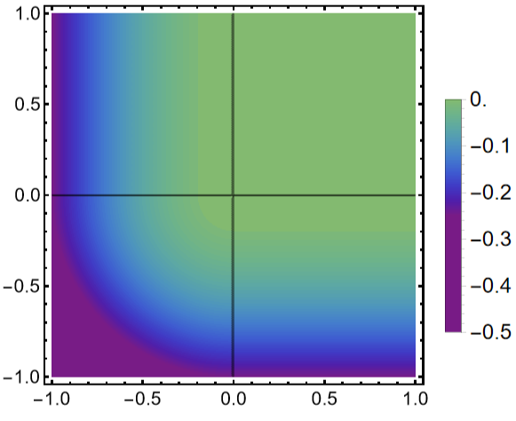
Phase diagrams in the , space: case η=0
a
p
a
a
Curves at which the different phases have the same energy are calculated and shown in the space
(,)
a
p
a
a
beta=1;eta=0.0;Phases0=ContourPlot[PAdiagram["PhaseNumber",AlphaP[xx],AlphaA[yy],beta,eta],{xx,-1.0,1.0},{yy,-1,1},PlotPoints100,PlotRangeAll,Contours{1,2,3,4},ContourLinesTrue,ContourShadingFalse,FrameStyleDirective[Black,Thick],BaseStyle{FontSize16,FontFamily"Arial"},ColorFunctionScalingFalse,ColorFunction(FourPhaseColors[#]&)];
Energyofthedifferentphasesiscalulatedandshowninthe(,)space
a
p
a
a
Energy0=ContourPlotPAdiagram["energy",AlphaP[xx],AlphaA[yy],beta,eta],{xx,-1,1},{yy,-1,1},PlotPoints50,(*PlotRange{Automatic,-},*)Contours100,ContourLinesFalse,ContourShadingTrue,FrameStyleDirective[Black,Thick],BaseStyle{FontSize16,FontFamily"Arial"},ColorFunction(ColorData["Rainbow"][#-0.5]&),PlotLegends->BarLegend[Automatic,None,LabelStyle->Directive[Black,FontSize18,FontFamily"Arial"],LegendLabel->""];
-12
10
Combined plots of energy and phases transition curves
In[]:=
Show[Energy0,Phases0]
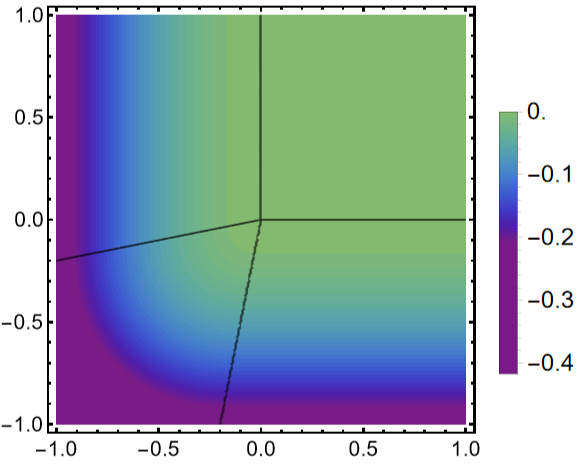
Phase diagrams in the , space: case η=0.2
a
p
a
a
In[]:=
(*Curvesatwhichthedifferentphaseshavethesameenergyarecalulatedandshowninthe(,)space*)beta=1;eta=0.2;Phases1=ContourPlot[PAdiagram["PhaseNumber",AlphaP[xx],AlphaA[yy],beta,eta],{xx,-1.0,1.0},{yy,-1,1},PlotPoints150,PlotRangeAll,Contours{1,2,3,4},ContourLinesTrue,ContourShadingFalse,FrameStyleDirective[Black,Thick],BaseStyle{FontSize16,FontFamily"Arial"},ColorFunctionScalingFalse,ColorFunction(FourPhaseColors[#]&)];
a
p
a
a
In[]:=
Energy1=ContourPlotPAdiagram["energy",AlphaP[xx],AlphaA[yy],beta,eta],{xx,-1,1},{yy,-1,1},PlotPoints50,(*PlotRange{Automatic,-},*)Contours60,ContourLinesFalse,ContourShadingTrue,FrameStyleDirective[Black,Thick],BaseStyle{FontSize16,FontFamily"Arial"},ColorFunction(ColorData["Rainbow"][#-0.5]&),PlotLegends->BarLegend[Automatic,None,LabelStyle->Directive[Black,FontSize18,FontFamily"Arial"],LegendLabel->""];
-12
10
Combined plots of energy and phases transition curves
In[]:=
Show[Energy1,Phases1]
Phase diagrams in the , space: case η=0.9
a
p
a
a
In[]:=
(*Curvesatwhichthedifferentphaseshavethesameenergyarecalulatedandshowninthe(,)space*)beta=1;eta=0.90;Phases2=ContourPlot[PAdiagram["PhaseNumber",AlphaP[xx],AlphaA[yy],beta,eta],{xx,-1.0,1.0},{yy,-1,1},PlotPoints150,PlotRangeAll,Contours{1,2,3,4},ContourLinesTrue,ContourShadingFalse,FrameStyleDirective[Black,Thick],BaseStyle{FontSize16,FontFamily"Arial"},ColorFunctionScalingFalse,ColorFunction(FourPhaseColors[#]&)];
a
p
a
a
In[]:=
Energy2=ContourPlotPAdiagram["energy",AlphaP[xx],AlphaA[yy],beta,eta],{xx,-1,1},{yy,-1,1},PlotPoints50,(*PlotRange{Automatic,-},*)Contours30,ContourLinesFalse,ContourShadingTrue,FrameStyleDirective[Black,Thick],BaseStyle{FontSize16,FontFamily"Arial"},ColorFunction(ColorData["Rainbow"][#-0.5]&),PlotLegends->BarLegend[Automatic,None,LabelStyle->Directive[Black,FontSize18,FontFamily"Arial"],LegendLabel->""];
-12
10
Combined plots of energy and phases transition curves
Combined plots of energy and phases transition curves
Polarization Loops of HfZrO2 films (Figure 3)
Polarization Loops of HfZrO2 films (Figure 3)
Polarization dependence on the external electric field is plotted using the function “Loops” with either static or dynamic output. It is either single or double hystereis loop for ferroelectric or antiferroelectric phases respectively
Film with h=10 nm (Figure 3: bottom row)
Film with h=10 nm (Figure 3: bottom row)
Combined loops
Film with h=20 nm (Figure 3: middle row)
Film with h=20 nm (Figure 3: middle row)
Film with h=30 nm (Figure 3: top row)
Film with h=30 nm (Figure 3: top row)
(x,h)- Phase-Diagram - Gaussian-type activation and Alpha-Plots (Figure 4-5)
(x,h)- Phase-Diagram - Gaussian-type activation and Alpha-Plots (Figure 4-5)
Phase diagram calculated with the help of the above - listed functions
Concentration Loops for HfZrO2 films (Figure 7)
Concentration Loops for HfZrO2 films (Figure 7)
In this subsection we consider 2D concentratin of the free carriers on the interface between ferroelectric and grahene monolayer. This concentration is related to ferroelectric polarization therefore its dependence on the external electric field could plotted using the function “Loops”
h = 10 nm (bottom row)
h = 10 nm (bottom row)
h=20 nm (middle row)
h=20 nm (middle row)
h=30 nm (top row)
h=30 nm (top row)
Supplements
Supplements
Test of loops
Test of loops
CITE THIS NOTEBOOK
CITE THIS NOTEBOOK
Charge-polarization coupling in the nanostructure thin HFxZr1-xO2 film-graphene
by Eugene A. Eliseev and Anna N. Morozovska
Wolfram Community, STAFF PICKS, May 17, 2024
https://community.wolfram.com/groups/-/m/t/3178088
by Eugene A. Eliseev and Anna N. Morozovska
Wolfram Community, STAFF PICKS, May 17, 2024
https://community.wolfram.com/groups/-/m/t/3178088