Wolfram Cloud Document

ABSTRACT (original article): Dice control involves “setting” the dice and then throwing them carefully, in the hope of influencing the outcomes and gaining an advantage at craps. How does one test for this ability? To specify the alternative hypothesis, we need a statistical model of dice control. Two have been suggested in the gambling literature, namely the Smith-Scott model and the Wong-Shackleford model. Both models are parameterized by

θ∈[0,1]

, which measures the shooter’s level of control. We propose and compare four test statistics: (a) the sample proportion of 7s; (b) the sample proportion of pass-line wins; (c) the sample mean of hand-length observations; and (d) the likelihood ratio statistic for a hand-length sample. We want to test

:θ=0

(no control) versus

:θ>0

(some control). We also want to test

:θ≤

versus

:θ>

, where

is the “break-even point.” For the tests considered we estimate the power, either by normal approximation or by simulation. CITATION (original article): Stewart N. Ethier(2025), Testing for dice control at craps, arXiv:2504.13158. https://doi.org/10.48550/arXiv.2504.13158

This notebook implements computational methods to analyze dice control in craps using two statistical models: the Smith–Scott (S–S) and Wong–Shackleford (W–S) models. It reparameterizes these models via the expected gain η from a pass-line bet, enabling hypothesis testing for dice-control efficacy. Key tasks include calculating eigenvalues of transition matrices, tail probabilities for hand lengths, and optimal strategies, as described in the paper’s theoretical framework.

Smith--Scott model

This section defines the Smith–Scott (S–S) model , which assumes a shooter reduces off-axis dice rolls by proportion theta ∈ [0, 1]. Functions like pA[x], pB[x], and pC[x] encode probability distributions for dice sets targeting specific face reductions. The code computes reparameterized probabilities pAA[x, theta], pAB[x, theta], etc., as per the paper’s modified S–S formulation, linking theta to the probability of rolling a 7 to test control effectiveness.

Definitions


Optimal strategy

In[]:=

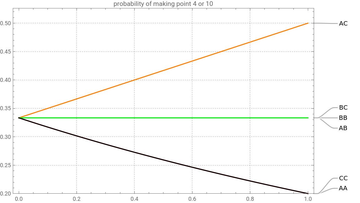
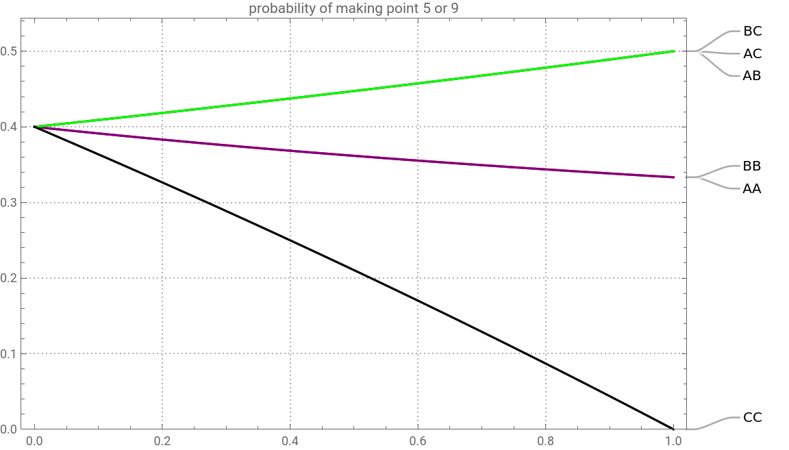
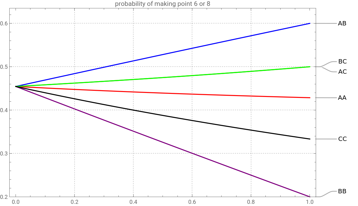
Plot[{pAA[4,theta]/(pAA[4,theta]+pAA[7,theta]),pAB[4,theta]/(pAB[4,theta]+pAB[7,theta]),pAC[4,theta]/(pAC[4,theta]+pAC[7,theta]),pBB[4,theta]/(pBB[4,theta]+pBB[7,theta]),pBC[4,theta]/(pBC[4,theta]+pBC[7,theta]),pCC[4,theta]/(pCC[4,theta]+pCC[7,theta])},{theta,0,1},PlotRange->{0.2,0.5},PlotStyle->{Red,Blue,Orange,Purple,Green,Black},PlotLabels{"AA ","AB ","AC ","BB ","BC ","CC "},PlotTheme->"Detailed",PlotLegends->None,PlotLabel->"probability of making point 4 or 10",ImageSize->Large]Plot[{pAA[5,theta]/(pAA[5,theta]+pAA[7,theta]),pAB[5,theta]/(pAB[5,theta]+pAB[7,theta]),pAC[5,theta]/(pAC[5,theta]+pAC[7,theta]),pBB[5,theta]/(pBB[5,theta]+pBB[7,theta]),pBC[5,theta]/(pBC[5,theta]+pBC[7,theta]),pCC[5,theta]/(pCC[5,theta]+pCC[7,theta])},{theta,0,1},PlotRange->{0,0.5},PlotStyle->{Red,Blue,Orange,Purple,Green,Black},PlotLabels{"AA ","AB ","AC ","BB ","BC ","CC "},PlotTheme->"Detailed",PlotLegends->None,PlotLabel->"probability of making point 5 or 9",ImageSize->Large]Plot[{pAA[6,theta]/(pAA[6,theta]+pAA[7,theta]),pAB[6,theta]/(pAB[6,theta]+pAB[7,theta]),pAC[6,theta]/(pAC[6,theta]+pAC[7,theta]),pBB[6,theta]/(pBB[6,theta]+pBB[7,theta]),pBC[6,theta]/(pBC[6,theta]+pBC[7,theta]),pCC[6,theta]/(pCC[6,theta]+pCC[7,theta])},{theta,0,1},PlotRange->{0.2,0.6},PlotStyle->{Red,Blue,Orange,Purple,Green,Black},PlotLabels{"AA ","AB ","AC ","BB ","BC ","CC "},PlotTheme->"Detailed",PlotLegends->None,PlotLabel->"probability of making point 6 or 8",ImageSize->Large]Plot[{pAA[7,theta]+pAA[11,theta]+2pAA[4,theta]pAC[4,theta]/(pAC[4,theta]+pAC[7,theta])+2pAA[5,theta]pAC[5,theta]/(pAC[5,theta]+pAC[7,theta])+2pAA[6,theta]pAB[6,theta]/(pAB[6,theta]+pAB[7,theta]),pAB[7,theta]+pAB[11,theta]+2pAB[4,theta]pAC[4,theta]/(pAC[4,theta]+pAC[7,theta])+2pAB[5,theta]pAC[5,theta]/(pAC[5,theta]+pAC[7,theta])+2pAB[6,theta]pAB[6,theta]/(pAB[6,theta]+pAB[7,theta]),pAC[7,theta]+pAC[11,theta]+2pAC[4,theta]pAC[4,theta]/(pAC[4,theta]+pAC[7,theta])+2pAC[5,theta]pAC[5,theta]/(pAC[5,theta]+pAC[7,theta])+2pAC[6,theta]pAB[6,theta]/(pAB[6,theta]+pAB[7,theta]),pBB[7,theta]+pBB[11,theta]+2pBB[4,theta]pAC[4,theta]/(pAC[4,theta]+pAC[7,theta])+2pBB[5,theta]pAC[5,theta]/(pAC[5,theta]+pAC[7,theta])+2pBB[6,theta]pAB[6,theta]/(pAB[6,theta]+pAB[7,theta]),pBC[7,theta]+pBC[11,theta]+2pBC[4,theta]pAC[4,theta]/(pAC[4,theta]+pAC[7,theta])+2pBC[5,theta]pAC[5,theta]/(pAC[5,theta]+pAC[7,theta])+2pBC[6,theta]pAB[6,theta]/(pAB[6,theta]+pAB[7,theta]),pCC[7,theta]+pCC[11,theta]+2pCC[4,theta]pAC[4,theta]/(pAC[4,theta]+pAC[7,theta])+2pCC[5,theta]pAC[5,theta]/(pAC[5,theta]+pAC[7,theta])+2pCC[6,theta]pAB[6,theta]/(pAB[6,theta]+pAB[7,theta])},{theta,0,1},PlotRange->{0.45,0.7},PlotStyle->{Red,Blue,Orange,Purple,Green,Black},PlotLabels{"AA ","AB ","AC ","BB ","BC ","CC "},PlotTheme->"Detailed",PlotLegends->None,PlotLabel->"probability of winning pass-line bet, assuming optimal dice sets on point rolls",ImageSize->Large]

Out[]=

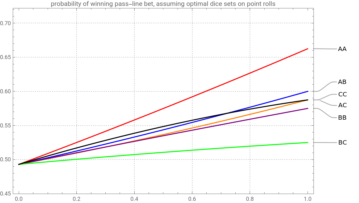
Conclude optimal strategy is AC if point is 4, 5, 9, or 10, and AB if point is 6 or 8, AA on come-out rolls.

Expected gain

In[]:=

EG[theta_]:=2(pAA[7,theta]+pAA[11,theta]+pAA[4,theta]pAC[4,theta]/(pAC[4,theta]+pAC[7,theta])+pAA[5,theta]pAC[5,theta]/(pAC[5,theta]+pAC[7,theta])+pAA[6,theta]pAB[6,theta]/(pAB[6,theta]+pAB[7,theta])+pAA[8,theta]pAB[8,theta]/(pAB[8,theta]+pAB[7,theta])+pAA[9,theta]pAC[9,theta]/(pAC[9,theta]+pAC[7,theta])+pAA[10,theta]pAC[10,theta]/(pAC[10,theta]+pAC[7,theta]))-1;theta=.;Factor[EG[theta]]

Out[]=

-448+10064theta-72

theta

-68

theta

72(-10+theta)(44+theta)

In[]:=

rho[theta_]:=-

-448+10064theta-72

theta

-68

theta

72(-10+theta)(44+theta)

;NSolve[rho[theta]==0,theta]

Out[]=

{{theta66.8253},{theta12.8481},{theta-11.7179},{theta0.0445299}}

In[]:=

Plot[rho[theta],{theta,0,1}]rho[0]rho[1]

Out[]=

Hand length mean and variance

Eigenvalues of transition matrix

Eigenvectors of transition matrix

Replace Root4 above by 144e1, Root3 by 144e2, Root2 by 144e3, and Root1 by 144e4.

Eigenvectors for non-unit eigenvalues are of the form ...

Characteristic polynomial of Q

Alternative form for non-unit eigenvalues

List the polynomials appearing in the above solutions

Example to illustrate theorem

Wong--Shackleford model

This section implements the Wong–Shackleford (W–S) model , which assumes correlated dice outcomes without favoring on-axis rolls. Functions like q4[a,b,c,d,theta], q5[...], and q6[...] calculate the probability of making the point 4 (or 5 or 6) given the dice set (a,b,c,d) and theta. These align with the paper’s reparameterization of theta to unify comparisons with the S–S model, enabling analysis of optimal betting strategies and statistical power under both frameworks.