This notebook series is designed to introduce selected dynamic economic models to both advanced undergraduate and graduate students. Economists have relied on a series of economic models to better understand the otherwise highly complex causal relationship among many economic variables. Dynamic economic models set up by systems of either difference or differential equations are particularly useful in tracing the change in the quantity of unknown economic variables (e.g., the capital stock, demand for labor, aggregate output, etc.) and their interactions over time.
This notebook series aims to help students better understand the depth, usefulness, and limitations of major existing micro and macroeconomic models by demonstrating how we can use Wolfram Mathematica to replicate and reconstruct the core ideas and find dynamic solution of the model.
The model introduced in this notebook series include, among others, (1) the cobweb model of the quantity and price adjustment, (2) Keynes’s aggregate demand model, (3) Hicks’s ISLM model, (4) Samuelson’s investment accelerator model, (5) Kalecki’s investment delay model, (6) the predator-prey interaction model, (7) the epidemic model, (8) Ricardo’s three dimensional business cycle model, (9) Marx-Goodwin business cycle and growth model, (10) Smith’s and Ricardo’s growth model, (11) the Harrod-Domar growth model, (12) the Solow growth model, (13) the RBC model, (14) Romer’s new growth model, and (15) the circuit of capital model.
Dynamic inflation models I
Smith’s and Ricardo’s theory of money and price
Smith’s and Ricardo’s theory of money and price
Introduction
Introduction
Inflation is an important economic phenomenon, in which the overall price level in an economy is continuously rising. The US federal government, the Bureau of Labor Statistics (BLS) specifically have conducted regular surveys on the price variable and presented the data for both consumer price index (CPI) and the producer price index (PPI).
If any of these indexes continues to rise for various reason, we can measure the rate of the change in this price index. The inflation rate is the growth rate of this measured price index over periods (monthly, quarterly, and annually). If the growth rate of this price level falls negative, we call it deflation, which is the opposite of inflation.
Why does the inflation-deflation occur? What are the cause of this continuous rise and fall in the measured price index? Economists disagree with one another about the fundamental cause of this inflation/deflation phenomenon. In this note, we present the most representative inflation models.
One useful reference for classifying various inflation theories is to make a distinction between (1) the quantity of money theory of inflation and (2) the cost of production theory of inflation. The modern day revival of the classical quantity of money theory of inflation is better known as ‘monetarism’ or ‘monetarist theory of inflation.’
From the perspective of history of economic thoughts, the debate between these two camps goes back to the debate between Adam Smith’s and David Hume-David Ricardo’s respective theory of money and price. Smith argued that the inflow of money (i.e., gold and silver) could be used to finance the operation of manufacture, thereby further stimulating economic activity, without causing any substantial inflationary effect.
David Hume and David Ricardo, on the other hand, maintained the position that the inflow of gold and silver or domestic banks’ disproportional increase in the quantity of paper money (banks’ bill of exchange, for example) would drive up the price level, thereby increasing the inflation rate. Smith’s position toward the effect of monetary flow became a foundation of British Banking School, whereas Hume-Ricardo’s stance formed the basis of British Currency School.
Later economists have adopted in one way or another some aspects of this classical debate between Smith and Ricardo. For example, Cagan and Friedman’s monetarist theory of inflation is a revival of Hume-Ricardo’s particular interpretation of the classical quantity of money equation (MV=PY), whereas Keynes and Post Keynesian economists’ cost of production approach to inflation is a lot more akin to Smith’s intuition about the positive effect of monetary flow on the increase in productive capacity.
In this note, we aims to reconstruct and present the most representative inflation models taught in advanced macroeconomics courses. For this purpose, this note is organized as follow: (1) In the first section, we present Smith’s and Ricardo’s respective theory of money and price using differential equation tools; (2) In the second section, we reconstruct Cagan and Friedman’s monetarist inflation model; (3) after briefly discussing Keynes’s cost of production theory of inflation in the third section, (4) we present the so-called wage-price spiral model as a special case of Keynes’s cost of production theory of inflation.
Smith’s theory of money and price
Smith’s theory of money and price
Introduction
Introduction
◼
Smith’s one important contribution is his ‘endogenous theory of money and bank.’ Here, the ‘money and bank’ is rather a metaphoric expression that encompasses the entire process of lending and borrowing. Smith does not provide any detailed analysis of forms of money and institutional characteristics of banks. Instead, he focuses on the effect of the change in the quantity of paper money issued by some lenders on the economy. The term ‘endogenous’ also has its unique meaning in the sense that the change in the quantity of paper money issued by private commercial banks is not determined by some arbitrary external factors but rather driven by internal logic of financial transactions such as the change in the demand for bank loans and the creditworthiness of borrowers in the economy.
◼
Smith lived in an era that the actual reserve and accumulation of gold and silver formed the basis of the dominant monetary and payment system. Even though other means of payment such as minted coins and paper money were circulated in a particular locality to facilitate various financial and business transactions, their circulation was fundamentally governed and regulated by the actual reserve (physical holding) of gold and silver stored in the vault of major influential private banks and the Bank of England.
◼
What would be the effect of the change in the gold reserve? What would happen if the quantity of paper money issued and circulated in the economy is increased? Smith maintains the optimistic view that the increase in paper money will have a positive impact on the nation’s productive capacity. The country’s capacity to produce and consume more goods will be enhanced if a greater quantity of paper money is issued by private banks and used to finance the investment project.
◼
To highlight this idea, this section presents a simple model of the change in the quantity of paper money and the change in the output in the economy, which captures the essence of Smith’s ideas on this issue.
The model structure and analytical solution
The model structure and analytical solution
◼
The specification of variables and parameter
Let us consider the change in the quantity of paper money, M, and the change in the country’s aggregate productive capacity measured by output, Y. The quantity of money at a given point in time, M(t) is a function of both inflow and outflow variable. If we assume that there is a certain fixed ratio of money that is newly issued and another ratio of settlement or repayment of the debt, we can write,
M
t
M
(
1
)If we temporarily ignore all the possible complications associated with making business loans (such as time delay in deal-making, perceived creditworthiness of borrowers, riskiness of business venture, etc), and if we assume that a certain fixed proportion of the loan is used to finance the setup and operation of the production activity, we can write another equation for the change in the aggregate output at time t, Y(t), as a function of the proportion of money devoted to the production activity as follows:
Y
t
Y
(
2
)In this formulation, cM(t) represents the amount or proportion of paper money that is used to finance the productive operation of new manufacturing activity, whereas (1-c)M(t) is the portion that is used to finance the consumption for “idle people.” To put it another way, the ‘investment (loan) ratio’ determines the proportion of business loans in the total private loans. By ‘idle people’, Smith meant those who live on collecting surplus income such as rents and interest rather than proactively engaging in the nation’s productive activity.
◼
The analytical solution of the model
These two differential equations constitute a model that describes the relationship between the change in output and the change in the volume of paper money, and its analytical solution can be found by:
In[]:=
Clear[sol,M,Y,M0,Y0,a,b,c,t];DSolve[{M'[t]==aM[t]-bM[t],Y'[t]==cM[t]-(1-c)M[t],M[0]==M0,Y[0]==Y0},{M[t],Y[t]},t]
Out[]=
M[t]M0,Y[t]
(a-b)t
M0-2cM0-M0+2cM0+aY0-bY0
(a-b)t
(a-b)t
a-b
The static visualization of the solution with fixed parameters
The static visualization of the solution with fixed parameters
Let us assign some arbitrary parameters to each of the following parameters and the initial value. The increase in the quantity of paper money stimulates the production and aggregate output as the significant portion of this new source of finance is used to facilitate and contribute to the production of output.
In[]:=
Clear[sol,M,Y,a,b,c,t];a=0.3;b=0.2;c=0.6;sol=NDSolve[{M'[t]==aM[t]-bM[t],Y'[t]==cM[t]-(1-c)M[t],M[0]==10,Y[0]==100},{M[t],Y[t]},{t,0,100}]
Out[]=
M[t]InterpolatingFunction[t],Y[t]InterpolatingFunction[t]


In[]:=
Plot[Evaluate[{M[t],Y[t]}/.sol],{t,0,100},PlotLegends->{"M(t)","Y(t)"}]
Out[]=
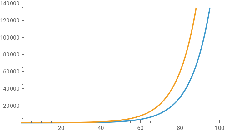


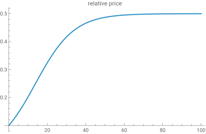
Let us now take the ratio of the quantity of paper money and the output. As we can see below, this ratio initially increases but is soon stabilized.
In[]:=
Plot[Evaluate[M[t]/Y[t]/.sol],{t,0,100},PlotLabel->"relative price"]
Out[]=
The interactive visualization of the solution curve
The interactive visualization of the solution curve
The following syntax allows us to see the dynamic and interactive charts. Both the solution curve of output change and paper money supply and their ratio can be analyzed as the value of the investment ratio changes.
In[]:=
ClearAll["Global`*"];a=0.3;b=0.2;sol1=ParametricNDSolve[{M'[t]==aM[t]-bM[t],Y'[t]==cM[t]-(1-c)M[t],M[0]==10,Y[0]==100},{M,Y},{t,0,100},{c}]
Out[]=
MParametricFunction,YParametricFunction

In[]:=
Manipulate[Plot[Evaluate[{M[c][t],Y[c][t]}/.sol1],{t,0,100}],{{c,0.6},0.5,0.8},SaveDefinitions->True]
Out[]=


In[]:=
Manipulate[Plot[Evaluate[M[c][t]/Y[c][t]/.sol1],{t,0,100}],{{c,0.6},0.5,0.8},SaveDefinitions->True]
Out[]=
Conclusion
Conclusion
◼
We have represented Smith’s endogenous theory of money and price in a simple mathematical model.
◼
There are several questions unanswered in Smith’s theory of money, bank, and price. First, Smith avoids asking an important question about the proper proportion between the actual gold reserve and the quantity of paper money issued by private banks. To what extent and how much of paper money can private banks print relative to the actual reserve of gold and silver in the economy? Isn’t there any desirable ratio between the two in the economy? Smith simply sets aside asking this question.
◼
Furthermore, Smith does not ask whether the relationship between the change in the quantity of paper money and the change in the country’s productive capacity can be possibly changing over time depending on how fast the same amount of paper money changes hands. To put it another way, Smith ignore the possible complication of the effect of the time-varying velocity of money.
◼
What would happen to the price level if the country can no longer use paper money in such a productive way to set up and operate new manufactures as described by Smith? What would happen, therefore, if a greater proportion of paper money is used to finance the “idle people’s” consumption binge?
◼
What about the probability of business failure? What would happen if new manufacturers face a significant shortfall in the demand for the goods that they have produced? If the increasing number of new startups fail to repay the debt, don’t we have a prolonged contraction in the availability of new loans in the economy?
Ricardo’s theory of money and price
Ricardo’s theory of money and price
Introduction
Introduction
◼
This section of note presents Ricardo’s contrasting theory of money and price. Ricardo’s theory of money and its effects on domestic price level shows that he is a true believer of a proto type ‘classical dichotomy’ and the monetarist theory of inflation better known as ‘the quantity of money theory of inflation.’
◼
The term classical dichotomy is the belief shared by many classical political economists. It stipulate the argument that the change in monetary variables (e.g., the quantity of money, the rate of interest, etc.) is unrelated with the change in non-monetary or real variables (e.g., the output, employment, etc). The the quantity of money theory of inflation is another superficial observation that the change in the price level or its rate of change (inflation) is always driven by the change in the quantity of money issued by domestic financial institutions (primarily by central bank).
◼
The classical dichotomy also implies that the economy is operating at its full employment level in the absence of the government’s artificial intervention in the private business activities and, therefore, the increase in the quantity of money or the change in the availability of bank loans only aggravates the inflationary pressure in the economy.
The model structure and analytical solution
The model structure and analytical solution
◼
The specification of variables and parameter
As before, let us consider the change in the quantity of paper money, M, and the change in the country’s aggregate productive capacity measured by output, Y. The quantity of money at a given point in time, M(t) is a function of both inflow and outflow variable. If we assume that there is a certain fixed ratio of money that is newly issued and another ratio of settlement or repayment of the debt, we can write,
Similarly, if we assume that there is a fixed ratio of both production and consumption, we can write another equation for the change in the aggregate output at time t, Y(t), as a function of its own level:
◼
The analytical solution of the model
These two differential equations constitute a model that describes the relationship between the change in output and the change in the quantity of paper money, and its analytical solution can be found by:
The static visualization of the solution curve
The static visualization of the solution curve
◼
The static visualization of the solution curve I
Suppose we have the following arbitrary parameters and initial conditions. The numerical solution and its solution curve will be:
Notice that both Y(t) and M(t) are exponentially growing, and they are not related with one another. Instead, the growth of Y(t) is independently determined by the net growth rate (c-d), just as the growth rate of M(t) is independently determined by its own net growth rate of money supply (a-b).
The ratio between M(t) and Y(t) that measures the relative magnitude of the quantity of money and/or the change in the price level can be a fixed quantity if all the parameters that govern the change in M(t) and Y(t) stay the same.
◼
The static visualization of the solution curve II
If a greater quantity of money is injected into the economy, however, the ratio will go up as follow:
The interactive visualization of the solution curve
The interactive visualization of the solution curve
This time let us create an interactive chart that allows us to control the value of selected parameters.
Conclusion
Conclusion
◼
This note replicates Ricardo’s classical quantity of money theory of inflation. Ricardo believed that the private sector economy is always operating at its full employment level, and he did not assign any proactive role played by private commercial banks; these banks simply act in response to the change in the central bank’s monetary policy. Therefore, the central bank’s misguided expansionary monetary policy simply translates into unnecessary and costly inflationary pressure without stimulating aggregate demand and output.
Reference
Reference
Smith, Adam. 1999 [1776]. An Inquiry into the Causes and Nature of the Wealth of Nations Book I-III. edited with an introduction and notes by Andrew Skinner, London: Penguin Books.
Ricardo, David. 1996 [1817]. Principles of Political Economy and Taxation, Amherst, New York: Prometheus Books (based upon the 3rd edition published in 1821).
CITE THIS NOTEBOOK
CITE THIS NOTEBOOK
Introduction to dynamic economic models: Dynamic inflation models I
by Hee-Young Shin
Wolfram Community, STAFF PICKS, December 17, 2025
https://community.wolfram.com/groups/-/m/t/3592661
by Hee-Young Shin
Wolfram Community, STAFF PICKS, December 17, 2025
https://community.wolfram.com/groups/-/m/t/3592661