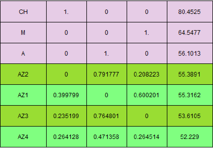
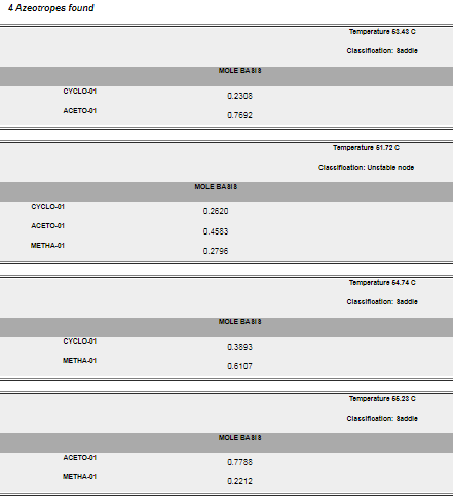
Let us consider a ternary mixture of cyclohexane, acetone, and methanol at . The vapor-liquid equilibrium (VLE) behavior is described by the modified Raoult's law with activity coefficients predicted by the Wilson model. This mixture presents seven azeotropes, whose locations and boiling points are given below: Aspen-Plus yields the following similar results :
101.325kPa
Cyclohexane = component 1
Acetone = component 2
Methanol = component 3
Acetone = component 2
Methanol = component 3
Total pressure (1 atm) in torr
In[]:=
P=760;
Wilson model
In[]:=
lambdas=Transpose@{{0,1016.11102294922,2298.60205078125},{305.441406250000,0,551.454528808594},{520.139221191406,-124.932800292969,0}};(*incal/mol*)volumes={108.8,74.0,40.7};(*inmL/mol*)wilson[x_,T_]:=Module[{Lambdas,gammas,i,j},For[i=1,i≤3,i++,For[j=1,j≤3,j++,Lambdas[i,j]=volumes[[j]]/volumes[[i]]*Exp[-lambdas[[i,j]]/(1.9872041*T)]]];For[i=1,i≤3,i++,gammas[i]=1-Log[Sum[Lambdas[i,k]x[[k]],{k,1,3}]];For[j=1,j≤3,j++,gammas[i]=gammas[i]-Lambdas[j,i]x[[j]]/Sum[Lambdas[j,k]x[[k]],{k,1,3}]]];Table[Exp[gammas[i]],{i,1,3}]]
Vapor pressure obtained using Antoine equation
In[]:=
A2=7.11714;B2=1210.595;C2=229.664;A1=4.13983+2.88081;B1=1316.554;C1=273.15-35.581;A3=8.08097;B3=1582.271;C3=239.726;myPsats={10^(A1-B1/(C1+(T-273.15))),10^(A2-B2/(C2+(T-273.15))),10^(A3-B3/(C3+(T-273.15)))};
System of algebraic equations, which solutions yield the azeotropes compositions and boiling point when λ=1
mysyshom[x_,T_,l_]:=Module[{gammas,psat},gammas=wilson[x,T];psat=myPsats;{x[[1]]-((1-l)+lgammas[[1]])psat[[1]]x[[1]]/P0,x[[2]]-((1-l)+lgammas[[2]])psat[[2]]x[[2]]/P0,x[[3]]-((1-l)+lgammas[[3]])psat[[3]]x[[3]]/P0,x[[1]]+x[[2]]+x[[3]]-10}]
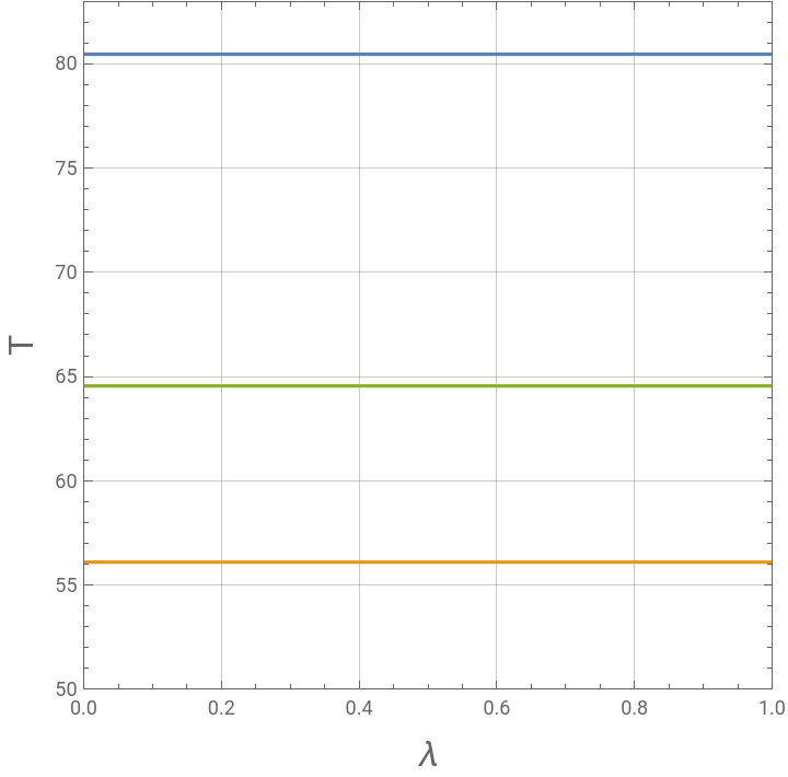
Pure components' boiling point versus λ
In[]:=
l=Table[i,{i,0,1,0.01}];data=.;guess={1,10^-12,10^-12,330};data[1]=Table[{l[[i]],-273.15+T/.FindRoot[mysyshom[{x1,x2,x3},T,l[[i]]],{x1,guess[[1]]},{x2,guess[[2]]},{x3,guess[[3]]},{T,guess[[4]]}]},{i,1,101}];guess={10^-12,1,10^-12,330};data[2]=Table[{l[[i]],-273.15+T/.FindRoot[mysyshom[{x1,x2,x3},T,l[[i]]],{x1,guess[[1]]},{x2,guess[[2]]},{x3,guess[[3]]},{T,guess[[4]]}]},{i,1,101}];guess={10^-12,10^-12,1,330};data[3]=Table[{l[[i]],-273.15+T/.FindRoot[mysyshom[{x1,x2,x3},T,l[[i]]],{x1,guess[[1]]},{x2,guess[[2]]},{x3,guess[[3]]},{T,guess[[4]]}]},{i,1,101}];p1=ListPlot[{data[1],data[2],data[3]},GridLinesAutomatic,FrameTrue,AspectRatio1,Joined->True,PlotRange{{0,1},{50,83}},FrameLabel{Style["λ",16],Style["T",16]}]
Out[]=
Compute the Jacobian matrix
In[]:=
x={x1,x2,x3};l=.;(*lisλ*)gammas=wilson[x,T];psat=myPsats;jac=Outer[D,{x[[1]]-((1-l)+lgammas[[1]])psat[[1]]x[[1]]/P,x[[2]]-((1-l)+lgammas[[2]])psat[[2]]x[[2]]/P,x[[3]]-((1-l)+lgammas[[3]])psat[[3]]x[[3]]/P,x[[1]]+x[[2]]+x[[3]]-1},{x1,x2,x3,T}];
Starting with the pure component mixture and track bifurcations
1st branch
1st branch
In[]:=
j=0;guessI={10^-12,10^-12,1.0,350};While[j≤501,k=1;guess=If[j0,guessI,guess];s=Quiet@FindRoot[mysyshom[{x1,x2,x3},T,(j)0.002],{x1,guess[[1]]},{x2,guess[[2]]},{x3,guess[[3]]},{T,guess[[4]]},MaxIterations10000];sol[j,1,1]=x1/.s;sol[j,2,1]=x2/.s;sol[j,3,1]=x3/.s;sol[j,4,1]=T/.s;jacs[j]=jac/.x1sol[j,1,1]/.x2sol[j,2,1]/.x3sol[j,3,1]/.Tsol[j,4,1]/.l(j)0.002;If[j≥2&&Sign[Det[jacs[j]]Det[jacs[j-1]]]<0,Print[j];eval=Eigenvalues[jacs[j]];pos=First@Position[Abs@eval,Min[Abs@eval]];evect=Flatten[Re[Eigenvectors[jacs[j]][[pos]]]];diff={0,0,0};inc=Exp@0.1;guess={x1,x2,x3,T}/.x1sol[j,1,1]/.x2sol[j,2,1]/.x3sol[j,3,1]/.Tsol[j,4,1];Print[Sign[Det[jacs[j]]Det[jacs[j-1]]]," ",pos," ",guess];k=1;While[Abs[diff[[1]]]<10^-5&&Abs[diff[[2]]]<10^-5&&Abs[diff[[3]]]<10^-5,{guess=Re@(guess+(incevect));s=Quiet@FindRoot[mysyshom[{x1,x2,x3},T,(j+1)0.002],{x1,guess[[1]]},{x2,guess[[2]]},{x3,guess[[3]]},{T,guess[[4]]},MaxIterations10000];nbw[1]=x1/.s;nbw[2]=x2/.s;nbw[3]=x3/.s;nbw[4]=T/.s;inc=-1.5inc;diff=Table[sol[j,i,1]-nbw[i],{i,1,3}],k++}];Table[sol[j,i,1]=nbw[i],{i,1,4}];];If[j≥2&&k≥2,Table[guess[[i]]=nbw[i],{i,1,4}],Table[guess[[i]]=sol[j,i,1],{i,1,4}]];j++]
25
-1 {4} {3.5×,0.,1.,337.698}
-323
10
26
-1 {4} {0.00639463,0.,0.993605,337.697}
In[]:=
dataaz1=Table[{j0.002,-273.15+sol[j,4,1]},{j,0,500,20}];
In[]:=
j=500;
In[]:=
d1={"AZ1",sol[j,1,1],sol[j,2,1],sol[j,3,1],sol[j,4,1]-273.15}//Chop
Out[]=
{AZ1,0.399799,0,0.600201,55.3162}
In[]:=
paz1=ListPlot[dataaz1,GridLinesAutomatic,FrameTrue,AspectRatio1,PlotMarkersStyle["■",Darker@Orange,12],PlotRange{{0,1},{52,66}}];
2nd branch
2nd branch
3rd branch
3rd branch
4th branch
4th branch
Pure components' boiling points
All seven azeotropes
Comparison with Matlab output
Acknowledgement
Acknowledgement
An analogous problem and its Matlab solution were developed and refined in the Chemical Engineering department at MIT by several people, including the late Prof. James Swan. Here, we provide the solution using Mathematica for a different ternary system.
CITE THIS NOTEBOOK
CITE THIS NOTEBOOK
All azeotropes for a ternary system by bifurcation: cyclohexane - acetone - methanol system
by Housam Binous and Ahmed Bellagi
Wolfram Community, STAFF PICKS, June 22, 2025
https://community.wolfram.com/groups/-/m/t/3483282
by Housam Binous and Ahmed Bellagi
Wolfram Community, STAFF PICKS, June 22, 2025
https://community.wolfram.com/groups/-/m/t/3483282