Simulating an Epidemic in Mathematica
Simulating an Epidemic in Mathematica
Eliza Kishan
ORCID: 0000-0001-7702-1676
King’s Interhigh, London, United Kingdom
King’s Interhigh, London, United Kingdom
Introduction
Mathematical modelling is a powerful tool used to study the spread and control of infectious diseases. By simulating an epidemic through mathematical models, researchers can estimate the potential impact of interventions, evaluate the effectiveness of public health policies, and predict the course of the epidemic over time. The recent COVID-19 pandemic has highlighted the importance of mathematical modelling in understanding and managing the spread of infectious diseases. Various mathematical models have been developed and used to forecast the spread of COVID-19, evaluate the impact of interventions such as lockdowns and social distancing measures, and estimate the potential number of cases, hospitalizations, and deaths. Through the use of mathematical models, researchers can gain valuable insights into the dynamics of epidemics and inform policy decisions to mitigate their impact. This project specifically does this, and takes a small set of variables in order to determine the spread of an epidemic. This is just converted into a small table in order to be a basic simulator.
Method
Using a modified SIR model, the epidemic will be simulated. The factors of susceptible subjects will be determined by a custom function described earlier. In this brief work, the specific described phenomena will be considerate of an average population. The SIR model is expressed as follows:
S(t)S(0)
-
R
0
R(t)-R(0)
N
e
S(0) is the initial number of susceptible subjects, R(0) is the initial number of removal subjects, N is the constancy of population, R0 is the basic reproduction number (popularly known as the R-not, a representation of how infective a pathogen is) , S(t) is the number of susceptible individuals as a function of time and R(t) is the number of removed individuals over time.
For this notebook, the general model will be for the Ebola virus for a unique perspective.
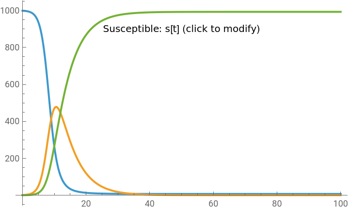
The SIR model is fairly simplistic, therefore, the graph produced will be fairly simplistic.
For this notebook, the general model will be for the Ebola virus for a unique perspective.
The SIR model is fairly simplistic, therefore, the graph produced will be fairly simplistic.
In[]:=
Manipulate[(*Definethedifferentialequations*)eqns={s'[t]==-b*s[t]*i[t],i'[t]==b*s[t]*i[t]-a*i[t],r'[t]==a*i[t]};(*Definetheinitialconditions*)ics={s[0]==s0,i[0]==i0,r[0]==r0};(*Definetheparametervalues*)params={a->aVal,b->bVal};(*Solvetheequations*)sol=NDSolve[{eqns,ics}/.params,{s,i,r},{t,0,100}];(*Plottheresults*)Plot[Evaluate[{s[t],i[t],r[t]}/.sol],{t,0,100},PlotRange->All,Epilog->{Text["Susceptible: "<>ToString[s[t]]<>" (click to modify)",{50,900}],EventHandler[Dynamic[Locator[Dynamic[{50,850}],Graphics[{Text[Style["Drag to change susceptible population",Blue,16],{50,850}],Text[Style["Current population: "<>ToString[Round[s[t]]],Black,12],{50,820}]},ImageSize->{300,100}],Appearance->None]],"MouseClicked":>InputField[Dynamic[s0],Number]]}],(*Definethesliders*){{aVal,0.2,"Recovery rate (a)"},0.01,1,0.01},{{bVal,0.001,"Infection rate (b)"},0.0001,0.1,0.0001},{{s0,999,"Initial susceptible population"},1,10000,1},{{i0,1,"Initial infected population"},1,10000,1},{{r0,0,"Initial recovered population"},0,10000,1}]
Out[]=


In[]:=