Out[]=
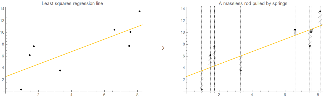
The problem of fitting a straight line through a set of points that don’t lie on a straight line has many proposed solutions with all sorts of different characteristics, yet one common feature of all these myriad methods is that they all try to find a line that is “in the middle” of the points. It’s as if each point had a little spring attached to it that tried to pull the line closer. In a wondrous coincidence, this turns out to be exactly how the least squares method operates. A physical system is in equilibrium when its potential energy is at a minimum. In the case of a zero-length spring (a spring for which tension is proportional to its length), potential energy is proportional to length squared. Consequently, for a system consisting of several identical zero-length springs, potential energy is proportional to the sum of the lengths of the springs squared. Now, imagine a set of zero-length springs fixed to a wall, each spring fixed at its own point. Each spring is impaled onto a long vertical shaft such that the free end can only move vertically. The free end of each spring is attached to a long lightweight (ideally massless) rod, and this is done in such a way that the point where each spring attaches to the rod can slide freely along the rod. The potential energy of this system is then proportional to the sum of the vertical distances squared, and as the system reaches equilibrium, the sum of the vertical distances squared is minimized. But this is exactly what the least squares line fit does! So the least squares method really does operate as if each point had a spring attached to it.
Out[]=


While this metaphor is somewhat of a spherical cow, it can actually be very helpful in understanding how high-leverage points affect the regression line. In the physical metaphor, the rod is in equilibrium when the total force and total torque acting on it are zero. Because of the first condition, the regression line must go through the center of mass of the points. Consider the second condition. Let’s say that there is a set of points that roughly lie on the same line, and we fit a least-squares regression line to them. In the illustration above, this is the orange line. Consider what happens when we add one more point to the far right of the initial cluster (shown in blue). The point literally has high leverage meaning that it’s positioned far from the center of mass, so even with a moderate remainder it can exert enormous torque on the rod, causing it to tilt significantly from the initial position. The blue point makes the regression line go almost directly through it, and the direction of the regression line is changed significantly even though the remainder of the blue point wasn’t even that large. There is a point with a larger remainder that nevertheless cannot pull the regression line closer because there are other springs balancing it out. As a side note, although the physical metaphor described above is unrealistic to implement in practice, it is not too hard to come up with a more practical alternative. Zero-length springs can be relaced with ordinary sprigs by fixing them not at the data points but a certain height lower, such that this extra difference in heights would compensate for the springs’ lengths. Instead of allowing all spring fixation points to slide freely on the rod, one of the springs should be attached to the rod directly in order to keep the rod from sliding out. With those changes, the setup appears to be completely realistic and could potentially be used at colleges and high schools as an illustration.
Code used to create the figures
Code used to create the figures
In[]:=
ClearAll[spring];spring[x_, y0_, y1_, n_, w_] := With[{s = (y1 - y0) / n}, Flatten@Table[Line[{{x, y0+s*i}, {x-w, y0+s*(i+1/4)}}], Line[{{x-w, y0+s*(i+1/4)}, {x+w, y0+s*(i+3/4)}}], Line[{{x+w, y0+s*(i+3/4)}, {x, y0+s*(i+1)}}], {i, 0, n-1}]];
In[]:=
Block[{data,model,a=2,b=1,xrange=10,npoints=8,errrange=4},data={#,a+b#+RandomReal[{-errrange,errrange}]}&/@Sort@Table[RandomReal[{0,xrange}],npoints];model=Normal@LinearModelFit[data,x,x];Row@{Show[{ListPlot[data,PlotStyleBlack],Plot[model,{x,0,xrange},PlotStyle->Blend[{Yellow,Orange}]]},ImageSize->Medium,PlotLabel->"Least squares regression line"],Style[" ",24],Show[{ListPlot[data,PlotStyle->Black],Plot[model,{x,0,xrange},PlotStyle->Blend[{Yellow,Orange}]],Graphics@Join[{Thin,Dashing[{0.003,0.003}],Line[{{#[[1]],-100},{#[[1]],100}}]}&/@data,{Gray,#}&/@Flatten[spring[#[[1]],#[[2]],(model/.x->#[[1]]),3,0.1]&/@data]]},ImageSize->Medium,PlotLabel->"A massless rod pulled by springs"]}]
In[]:=
Block[{data0,model0,data1,model1,a=1,b=0,xrange=10,npoints=8,errrange=1,p={30,2}},data0={#,a+b#+RandomReal[{-errrange,errrange}]}&/@Sort@Table[RandomReal[{0,xrange}],npoints];model0=Normal@LinearModelFit[data0,x,x];data1=Append[data0,p];model1=Normal@LinearModelFit[data1,x,x];Legended[Show[{Plot[model0,{x,0,p[[1]]},PlotStyle->Blend[{Yellow,Orange}]],Plot[model1,{x,0,p[[1]]},PlotStyle->{Dashed,Red}],ListPlot[data0,PlotStyle->Black],ListPlot[{p},PlotStyle->{Blue}],Graphics[{Gray,#}&/@Flatten[spring[#[[1]],#[[2]],(model0/.x->#[[1]]),3,0.15]&/@data1]]},ImageSize->Medium,PlotRange->{0,All}],LineLegend[{Blend[{Yellow,Orange}],Red},{"Original regression line","Line influenced by high leverage point (blue)"}]]]