Wolfram Cloud Document

Error Correcting Codes

Error correcting codes are an essential part of information theory and digital communication that enable reliable data transmission and storage. Error correcting codes help secure data during transmission through noisy channels and increase the reliability of data, allowing for error-free data transport in a range of applications such as deep space research, satellite broadcasting, mobile networks, and internet communication.

Channels

Error correcting codes convert bit streams of the original data into encoded streams to go through transmission channels. These channels are used to move data streams from one point to another. They can be in a physical form such as a wire or a non-physical form such as radios, mobile-phones, etc.

Noise

Noise and momentary electrical disturbances may cause changes in data as it passes through a communications channel. If the receiver fails to detect these changes, the received message will be incorrect, resulting in possibly serious consequences. As a first line of defense against data errors, these disturbances must be detected.

When we send a message online, say “Hi,” this message is converted into a binary form, which would be “1001,” before going through the transmission channel. Transition channels contain noise which may flip the bits of the binary code so that on the receiving end, we no longer receive our original message “1001” but instead may receive “1100” or “1011.” This binary code can no longer be traced back to get the original message “Hi”.

Here, error correction codes come into play.

Claude Shannon

Widely known as the “father of the information age,” Claude Shannon established channel capacity in his paper “A Mathematical Theory of Communication,” which states that for any given degree of noise contamination of a communication channel, it is theoretically possible to communicate discrete data (digital information) nearly error-free up to a computable maximum rate through the channel.

He begins by stating the pre-dominant issue:
"The fundamental problem of communication is that of reproducing at one point either exactly or approximately a message selected at another point”.

Channel capacity, also known as the Shannon Limit, showed that it is in fact possible to communicate at a positive rate and at the same time maintain a low error probability as desired. He proved the existence of such optimal error correcting codes. However, their construction is an ongoing process.

Linear Codes

Linear codes are a type of block code. To transmit a long data stream, the binary code is broken into bits of a fixed size. These groups of bits are known as blocks. Each type of block code has a generator matrix, which may be predefined or calculated. These generator matrices are used to encode the data stream by using their dot product with our actual message.

Parity Bits

Linear codes use parity bits as a method to protect data. Here, parity bits are previously defined bits added to the binary code. These are taken as “extra” bits which would help the transmission of the data if some bits are flipped by noise.

Generator Matrices

Linear codes are specified by a generator matrix, G. In some instances we can simplify G =



P. Here,



is the identity matrix of length k which determines the size of blocks into which the input data is divided, whereas P refers to the parity bits.

Hamming Distance

The Hamming distance between two codewords is the number of bits that are disparate between two bit strings.Typically, Hamming distance is denoted by the function d(x, y), where x and y are codewords. If we take the Hamming distance as H, the number of errors that our channel codes will be able to correct will always be less than half of H.

[Laplacian](x, y) = |{i|x

}|.

Encoding

We made an encoding function to protect the data bits from being flipped by noise in the channel.

This is the input binary message that will be used for our example.

In[]:=

input={0,0,1,1,1,1,0,0,0,0,1,1,1,0,1,0,0,1,1,1}

Out[]=

{0,0,1,1,1,1,0,0,0,0,1,1,1,0,1,0,0,1,1,1}

For linear codes, k is the length of the input blocks and n is the length of the code block we will generate once the message gets encrypted. As a rule, k is less than n.

To encode block codes, we multiply each block of binary message with the generator matrix.

In[]:=

encode[inp_List,Generator_List]:=Mod[Flatten[Part[inp,#].Generator&/@Range[Length[inp]]],2]

Decoding

Method

We decode the encoded data stream by creating a hash table. As we always know k, the length of original message, the hash table comprises all

binary combinations of that length as values and their

encoded versions as keys.

possibilities

creates a hash table of all possible messages the same length as our original message and assigns possible messages (values) to their encoded forms (keys).

In[]:=

possibilities[k_,g_]:=Module[{lengthMessage=k,gMatrix=g,hash=CreateDataStructure["HashTable"]},hash["Insert",Mod[#.gMatrix,2]->#]&/@Tuples[{1,0},lengthMessage];hash]

The minDistance function checks the minimum Hamming distance between all the possible messages of the length of original message.

In[]:=

minDistance[vectors_]:=Min[Select[Flatten[Table[HammingDistance[u,v],{u,vectors},{v,vectors}]],Positive]]

dec

odes

takes in the encoded blocks and the hash table. It then, compares each of the encoded blocks with all the possible encoded blocks and returns values (original messages) of the ones that exist in the hash table. If the encoded block is not found, the block is transferred to the notFound function, where each bit is changed until it matches an encoded block in the hash table. This change is done to find and fix errors.

In[]:=

notFound[b_List,s_]:=Module[{list1=b,list2=b,list3={}},Table[If[list2[[i]]==1,list2[[i]]=0,list2[[i]]=1];list3=Append[list3,list2];list2=list1;,{i,1,Length[b]}];If[s["KeyExistsQ",#],s["Lookup",#],Nothing]&/@list3]decodes[a_List,s_]:=If[s["KeyExistsQ",#],s["Lookup",#],Flatten[notFound[#,s]]]&/@a

Utilising Hamming Codes

Developed by R. W Hamming, Hamming codes are a type of block code with their own predefined generator matrix. These were the first codes in the family of block codes. They are able to detect up to two errors in the data stream and are able to correct one, with a relatively low redundancy. They are linear codes with excellent rate k/n≈ 1 but lower distance.

Herewearemakingageneratormatrixwhichaddsanidentitymatrix

totheHammingcodeParitybits-

In[]:=

MatrixForm[{{1,0,1},{1,1,1},{0,1,1},{0,1,0}}]

Out[]//MatrixForm=

1	0	1
1	1	1
0	1	1
0	1	0

Here we are taking the input message as hammingInput.

In[]:=

hammingInput={0,0,1,1,1,1,0,0,0,0,1,1,1,0,1,0}

Out[]=

{0,0,1,1,1,1,0,0,0,0,1,1,1,0,1,0}

Here hammingK is the length of the blocks we will be breaking the hammingInput into. As the Hamming Code Parity Bits have the dimensions 4 X3, k = 4.

In[]:=

hammingK=4

Out[]=

hammingStream is the hammingInput broken into blocks of length hammingK.

In[]:=

hammingStream=Partition[hammingInput,hammingK]

Out[]=

{{0,0,1,1},{1,1,0,0},{0,0,1,1},{1,0,1,0}}

We make the generator Hamming matrix using the makeGeneratorHammingmatrix function which adds to our hammingStrean, the Hamming parity bits and then transposes it.

makeGeneratorHammingMatrix[stream_List]:=Transpose[Join[IdentityMatrix[Length[stream]],Transpose[{{1,0,1},{1,1,1},{0,1,1},{0,1,0}}]]]generatorHammingMatrix=makeGeneratorHammingMatrix[hammingStream]

Out[]=

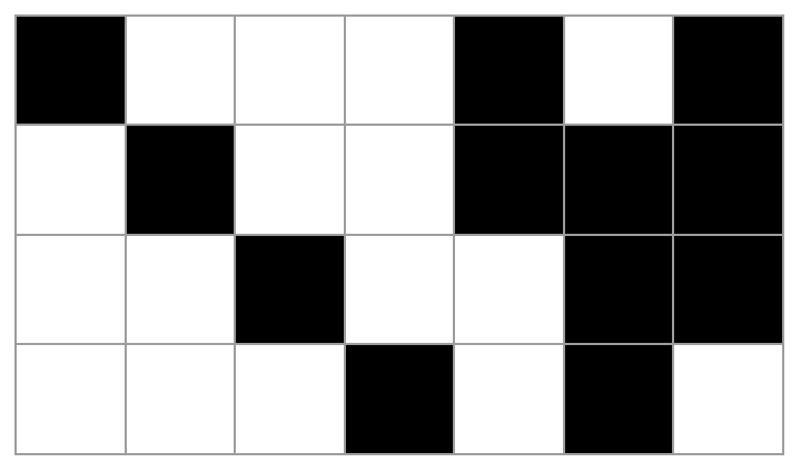
{{1,0,0,0,1,0,1},{0,1,0,0,1,1,1},{0,0,1,0,0,1,1},{0,0,0,1,0,1,0}}

Now we have received our Hamming Matrix. As this is our generator matrix of dimension kXn, k=4 and hammingN=7

In[]:=

MatrixForm[generatorHammingMatrix]

Out[]//MatrixForm=

1	0	0	0	1	0	1
0	1	0	0	1	1	1
0	0	1	0	0	1	1
0	0	0	1	0	1	0

In[]:=

hammingN=7

Out[]=

This is a visual of the generator Hamming matrix using ArrayPlot.

In[]:=

ArrayPlot[generatorHammingMatrix,Mesh->True]

Out[]=

We now get our encoded blocks using the encode function.

In[]:=

encodedHammingBlocks=encode[hammingStream,generatorHammingMatrix]

Out[]=

{0,0,1,1,0,0,1,1,1,0,0,0,1,0,0,0,1,1,0,0,1,1,0,1,0,1,1,0}

receivedHammingCodeword receives the encoded blocks after they have gone through a channel and may have flipped bits due to noise. It chops the data into blocks of length hammingN as this information is known to the decoder.

In[]:=

receivedHammingCodewords=Partition[encodedHammingBlocks,hammingN]

Out[]=

{{0,0,1,1,0,0,1},{1,1,0,0,0,1,0},{0,0,1,1,0,0,1},{1,0,1,0,1,1,0}}

hammingTable is the hash table containing all the possible messages of length hammingK and their encoded versions using the function possibilities.

In[]:=

hammingTable=possibilities[hammingK,generatorHammingMatrix]

Out[]=

DataStructure

Type:HashTable

Length:16



As minDistance is 2, this tells us that this specific message cannot correct any errors.

In[]:=

minDistance[hammingTable["Keys"]]

Out[]=

decodedHammingBlocks gives us the hammingStream again by decoding the receivedHammingCodewords by using the decodes function.

In[]:=

decodedHammingBlocks=Flatten[decodes[receivedHammingCodewords,hammingTable]]

Out[]=

{0,0,1,1,1,1,0,0,0,0,1,1,1,0,1,0}

To confirm the initial message and decoded message are the same-

In[]:=

SameQ[decodedHammingBlocks,hammingInput]

Out[]=

True

Hadamard Codes

Developed by Jacques Hadamard, Hadamard codes are block codes with their own pre-defined generator matrix.The Hadamard code is a code with extremely low rate but high distance. It is always used for error detection and correction when transmitting messages over very noisy or unreliable channels.

Implementation

Here we are taking the input message as hadamardStream.

hadamardInput here is the input stream broken into blocks of length hadamardK

Here is the constructor of the Hadamard code generator matrix as per the article below (this is not the same as the built-in function HadamardCode)

https://en.wikipedia.org/wiki/Hadamard_code

We make the generator Hadamard Matrix using the makeReducedgeneratorhadamardMatrix function which adds to our hadamardInput, the Hadamard parity bits and then goes on to transpose it.

Now we have received our Hadamard matrix. As this is our generator matrix of dimension kXn, k=3 and hadamardN=4

This is a visual of the Hadamard matrix.

encodedHammard is the encoded version of the hadamardInput.

receivedhadamardCodeword receives the encoded blocks after they have gone through a channel and may have flipped bits due to noise. It chops the data into blocks of length hammardN as this information is known to the decoder.

haddamardTable is the hash table containing all the possible messages of length hadamardk and their encoded versions using the function possibilities.

As the mindistance is 2 for this specific message, we cannot correct any error.

decodedhadamardBlocks decodes the receivedhadamardCodewords using the decodes function.

To confirm the initial message and decoded message are the same-

Reed Muller Codes

Reed Muller codes are a type of block codes who do not have a pre-defined generator matrix. One of the simplest and oldest error-correction codes, they are used for.............................. Reed Muller codes are defined as R[m,r] where ‘m’ gives us the number of variable to be included in our polynomials and ‘r’ tells us the degree of the polynomials. It uses polynomials as rules to encode blocks. Reed Muller codes are able to correct a mutable amount of error depending on the values of ‘m’ and ‘r.’

Implementation

Here, we are taking input as our original message.

variables creates a list of the polynomial which will be used including the constant polynomial, the number of variables pertaining to m, and the degree according to r.

binaryMaker takes the integer b and creates a list of ascending binary polynomials, with each element of length b.

kFromMR gives the length all input blocks should have, using m and r.

For our example, let us take m=3 and r=1

To get our message, we chop the input into blocks of length reedK.

assignPolynomials[] assigns all the polynomials (that we have received from variables,) their values.

rmMatrix is the Generator Reed Muller Matrix and uses the generatorRMMatrix function.

Here, we have a visual of the Generator Reed Muller Matrix.

Here we are multiplying the initial message with the generator matrix to get the encoded blocks.

receivedBlocks receives the encoded blocks after they have gone through a channel and may have flipped bits due to noise. It chops the data into blocks of length Power[2,m] (as is the formula).

rmTable is the hash table containing all the possible messages of length reedk and their encoded versions using the function possibilities.

As the minDistance is 4, we can correct one error.

decodedRMBlocks decodes the receivedBlocks using the decodes function.

To confirm the initial message and decoded message are the same-

Convolutional Codes

Developed in 1955 by Peter Elias, convolutional codes are a different type of linear codes who do separate the data into blocks but instead transmit the data stream as a long sequence using a continuous Shift Register. In the encoder, data bits are input to a Shift Register. As each bit enters at the left of the register, the previous bits are shifted to the right while the oldest bit in the register is removed. The number of error they can correct is dependent on the length of their Shift Register.

Implementation

messageC is the input message we are using.

The buffer is used in Convolution Codes as a default setting for the Shift Register. The makeBuffer creates the buffer according to user input.

Give your own input here. The input here must be the constant dimension.

Here, we have defined our polynomial rules. We can change these as long as the the dimensions are constant.

The stream is the message with the buffer included.

Here, we make the Shift Register. We have created the Shift Register as separate element for the code, however, it is in reality a continuous stream of data.

encpardy was our first encoding function for encoding the shiftRegisterList. encpardy computes the dot product of each element of the shiftRegisterList with each polynomial to give us our encoded message.

2nd version
encpardy2 was the second attempt at the encoding function. It produces the same output but is more efficient and simple as it does not require the use of the Transpose function.

The output is the encoded message.

makeBlocks receives the encoded blocks after they have gone through a channel and may have flipped bits due to noise. It chops the data into blocks of length of the constant dimension.

noisycodes here is an example of codewords with each element having its last 2 bits flipped.

insert is a function which flips the last bit of the list (shiftR) with the bit it receives as its second input.

dec is our decoding function for convolutional codes. It takes in codeword as the first input which is initially the buffer, shiftRegister as the second input which iterates over the list of the received codeWords and the rules which are the polynomials as its the third input. It creates two versions of the Shift Register Element (one ending with the bit - 0 and the other with the bit - 1). Next, it calculates the Hamming Distance between both these versions with the original codeword and returns the version with the smaller Hamming Distance. This output becomes the new codeword for the next element of the Shift Register.

decodedSR gives us the decoded output by removing the two extra buffer we had used for our computation in the earlier steps.

To confirm the initial message and decoded message are the same-

Turbo Codes

Turbo Codes are only error correction codes to exist which have come close approach the maximum channel capacity or Shannon limit. Introduced in the paper, “Near Shannon Limit Error-correcting Coding and Decoding: Turbo-codes”, in 1933, their results were not believed by several expert of the field.

Visualizations

A string is converted to ascii (8 bits) and flattened into our bit stream representation (list of 0’s ad 1’s).

This is the inverse operation (bits to text).

We simulate a noisy channel by flipping each bit with probability p. Note that according to Shannon there is still usable information unless p = 1/2.

We need to add a general function that takes in a type of code, a bitstream and whether we want to encode or decode and returns the coded (or decoded) stream. Here is a dummy version that simply flips all he bits (for encode and decode).

Finally, we have a UI where you can test all these codes yourself

Future Work

Turbo codes use encode the data stream in three steps. The data stream firstly gets encoded by a Recursive Systematic Coders (RSC), then goes through an Interleaver which randomly changes the positions of the data bits and finally passes through another RSC. After going through the channel and received by the decoder, it is transferred in a loop between two decoder which use soft decisions.