An important update of BIOKMOD is available: http://oed.usal.es/webMathematica/Biokmod/
Abstract
Abstract
BIOKMOD (http://oed.usal.es/webMathematica/Biokmod/) is a web application specially oriented to modeling the distribution of radioactive isotopes in the human body and animals, which includes some of the new ICRP models. The user himself can build biokinetic models, calculate the disintegrations produced in a compartment or organ, even adjust some of the model parameters to experimental data.
BIOKMOD uses compartmental modeling that involves the use of differential equations. Some of the most common isotopes used in Medicine and in the Nuclear Industry are built-up. But also, the user can build biokinetic models in an easy way, the researcher focuses on the construction of the model through a simple interface, the program automatically generates the differential equations and solves them, giving (if possible) the analytical expression and graphic representations.
To use BIOKMOD just a browser in any device (computer, tablet, smartphone) is needed. BIOKMOD is developed in the Wolfram Language (Mathematica) and is installed in a server where the computation is made. PDF version of the user manual: http://oed.usal.es/webMathematica/Biokmod/Docs/BIOKMOD_MANUAL.pdf
If you have Mathematica installed you can run the BIOKMOD packages in a Mathematica environment. The packages are available at: http://oed.usal.es/webMathematica/Biokmod/Docs/Biokmod20250411.zip
Introduction
Introduction
BIOKMOD has been enhanced for a long time since the initial version. It was developed for applications to workers exposed to radioactive intakes, but it has been expanded to include application in nuclear medicine. BIOKMOD kernel is developed using the Wolfram Language (former known as Mathematica). It is hosted on a web server. The user only needs a browser (e.g. Edge, Google Chrome, Firefox, …) to run the application.
It has a very simple interface that can be used by practitioners and non-specialist people without any knowledge of the Wolfram Language. The user himself can build biokinetic models, calculate the retention and the disintegrations produced in a compartment or organ, even adjust some of the model parameters to experimental data. Also, BIOKMOD includes the models of some isotopes most used in medicine and in the nuclear industry.
It has a very simple interface that can be used by practitioners and non-specialist people without any knowledge of the Wolfram Language. The user himself can build biokinetic models, calculate the retention and the disintegrations produced in a compartment or organ, even adjust some of the model parameters to experimental data. Also, BIOKMOD includes the models of some isotopes most used in medicine and in the nuclear industry.

Many of the example here includes can be made in the Mathematica environment. In this cases some BIOKMOD packages should be installed in Mathematica Applications folder.
In[]:=
Needs["Biokmod`SysModel2`"]
SysModel, version 2.1.1 2025-03-26
In[]:=
Needs["Biokmod`OIRModels`"]
OIRModels 1.3 2024-11-28
Compartmental models
Compartmental models
Compartmental modeling is one of the main application of BIOKMOD.
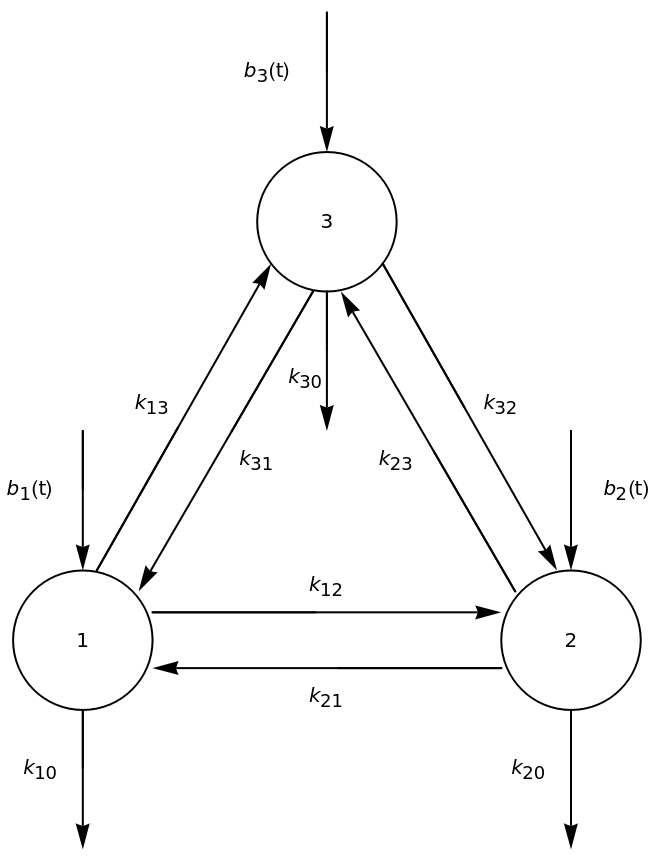
A generalized there compartmental models is shown below
Out[]=
x
1
k
10
k
12
k
13
x
1
k
21
x
2
k
31
x
3
b
1
x
2
k
12
x
1
k
20
k
21
k
23
x
2
k
32
x
3
b
2
x
3
k
13
x
1
k
23
x
2
k
30
k
31
k
32
x
3
b
3
The model can be expressed in matrix notation as follows:
x
(
1
)Being A the compartmental matrix where is a column vector representing the contents of the compartments:
x(t)
The function CompartMatrix[n, matrixA, λ] that returns the matrix of coefficients of a compartmental system, where n is the number of compartments of the system, matrixA represents the transfer rates, and λ is the radioactive decay constant (by default λ = 0, which means that it is not a radioactive isotope.).The transfer rates from compartment i to compartment j are written: {{1, 2, }, ..., {i, j, , ...}, by default = 0.
k
ij
k
12
k
ij
k
ij
In[]:=
CompartMatrix[3,{{1,1,k11},{1,2,k12},{2,2,k22},{2,3,k23},{3,3,k33},{2,0,k20}},λ]//MatrixForm
Out[]//MatrixForm=
-k12-λ | 0 | 0 |
k12 | -k20-k23-λ | 0 |
0 | k23 | -λ |
The solution of eq(1) when the coeffs are constants is Eq(2)
a
ij
x(t)=Exp(At)+[Exp(t-τ)A]b(τ)τ Eq(2)
x
0
t
∫
0
(
2
)The exponential matrix Exp(A t) can be build using the Mathematica function MatrixExp
For solving eq.(1) (with constants) the package has the function SystemDSolve. It applies, by default, an method developed by the author, based in eq(2), usually faster that the Mathematica build-up function DSolve. The package also gives the option so that the user can choose other methods.
a
ij
◼
SystemDSolve[A, IC, B(t), t, t1, x, options] gives the solution X(t)= {(t), ..., (t) at time t1 of an ODE system X'(t) = A X(t) + B(t), with initial conditions X(0) = IC , where the coeffsmatrix A = {{,..., }, ...,{, ..., }}; IC = {,.., , .}; B(t) ={[t],...,[t]}; x is the symbol that represents X; with options can be choose the method applied for solving the SODE, by default is apply: Method-> Automatic, other methods are LaplaceTransform, EigenValues, is applied the Eigenvalues-eigensisystem method, and DSolve is applied the Mathematica function DSolve.
x
1
x
n
a
11
a
1n
a
n1
a
nn
c
1
c
i
..,
c
n
b
1
b
n
◼
To solve (t)=Ax(t),t≥0 with i.c.: can be used SystemDSolve, however it is faster AcuteInput
x
x(0)=
x
0
◼
AcuteInput[A, IC,t1, x] or AcuteInput1[A, IC,t1, x] give the solution X(t)= {x1(t), ..., xn(t) at time t1 of an ODE system X'(t) = A X(t) , with initial conditions X(0) = IC
AcuteInput[matrixA_?MatrixQ, input_List, t_, x_] :=
Module[{r}, r = Dot[MatrixExp[matrixA t], input];
Thread[Subscript[x, #1][t] & /@ Range[Length[input]] -> r]];
AcuteInput1[matrixA_?MatrixQ, input_List, t_, x_] :=
Module[{r}, r = Dot[matrixExp[matrixA, t], input];
Thread[Subscript[x, #1][t] & /@ Range[Length[input]] -> r]];
Module[{r}, r = Dot[MatrixExp[matrixA t], input];
Thread[Subscript[x, #1][t] & /@ Range[Length[input]] -> r]];
AcuteInput1[matrixA_?MatrixQ, input_List, t_, x_] :=
Module[{r}, r = Dot[matrixExp[matrixA, t], input];
Thread[Subscript[x, #1][t] & /@ Range[Length[input]] -> r]];
◼
Tiacdes[unit of time: {sec, min, hour, day}, unit response functions {u1(t), ....uk(t)} (that it is the retention in each compartment assuming an single input 1 at t =0 in compartment i) , t, moment of time to be computed the accumulated disintegrations{t1, ..., tj} ] gives the Time integrated activity coefficients (TIAC) and the Time integrated activity or cumulative disintegration according to the MIRD definitions.
◼
Example.-This below model represents a three compartmental model where are the transfer coeffs. An input from out site of the system to compart. 1 and and ouput from compart. 1 to outside are consided.
k
ij
b
1
k
10
Out[]=
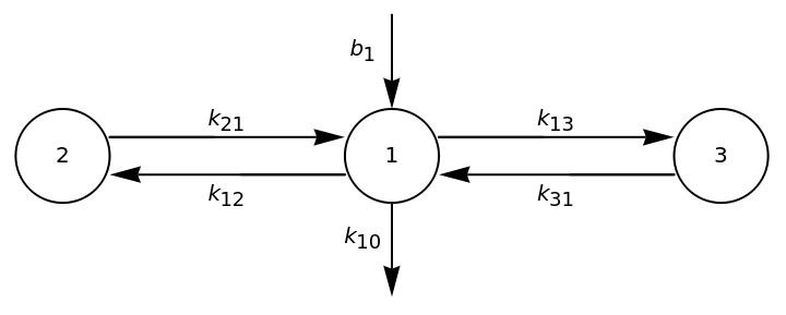
The coefficient transfer values, in , are = 0.01, =0.00798 , = 0.02, = 0.00272 and = 00230. An input b1= 1, in t = 0 is assumed ( it is equivalent to take as initial condition (0)= 1, (0)=(0) =0) of and isotope with decay constant, in , of 0.00012 ( If a stable element is considered this value is omitted.)
-1
min
k
12
k
21
k
13
k
31
k
10
x
1
x
2
x
3
-1
min
In[]:=
compartmatrix=CompartMatrix[3,{{1,2,0.01},{2,1,0.00798},{1,3,0.02},{3,1,0.00272},{1,0,0.0230}},0.00012]
Out[]=
{{-0.05312,0.00798,0.00272},{0.01,-0.0081,0.},{0.02,0.,-0.00284}}
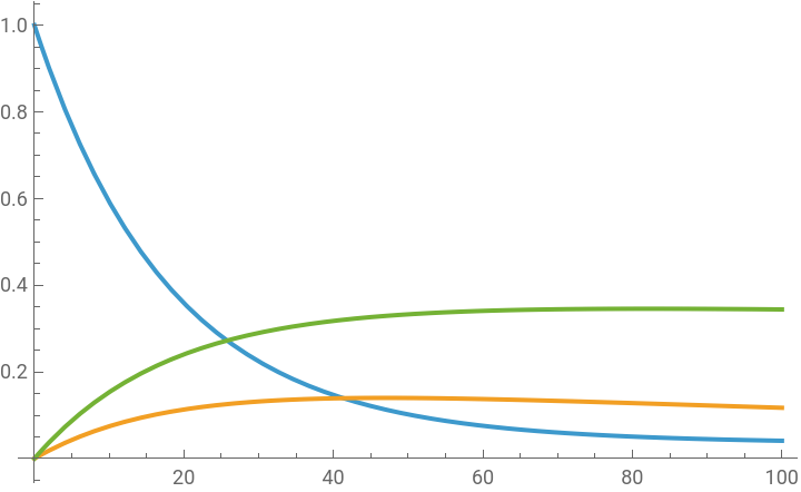
Then the impulse retention function in each compartments as function of the time (in min) assuming a single input 1 in t= 0 in compartment 1 is:
In[]:=
sol1=AcuteInput[compartmatrix,{1,0,0},t,x]//Simplify
Out[]=
{[t]0.948383+0.0200436+0.0315731,[t]-0.198743+0.151143+0.0476003,[t]-0.358022-0.101903+0.459924}
x
1
-0.0558191t
-0.00677386t
-0.00146703t
x
2
-0.0558191t
-0.00677386t
-0.00146703t
x
3
-0.0558191t
-0.00677386t
-0.00146703t
In[]:=
Plot[Evaluate[{[t],[t],[t]}/.sol1],{t,0,100},PlotLegendsAutomatic]
x
1
x
2
x
3
Out[]=


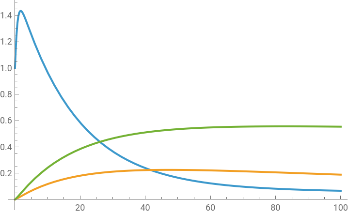
In this case it is also assumed and input to compart 1 given by:
0.1
t
-1.5t
e
In[]:=
sol2=SystemDSolvecompartmatrix,{1,0,0},,0,0,t,t1,x//ExpandAll
0.1
t
-(1.5t)
Out[]=
{[t1]0.948383+0.6022+0.0200436+0.0122681+0.0315731+0.0192497-0.632995Gamma[1.1,1.44418t1]-0.0128955Gamma[1.1,1.49323t1]-0.0202341Gamma[1.1,1.49853t1],[t1]-0.198743-0.126197+0.151143+0.0925102+0.0476003+0.0290213+0.13265Gamma[1.1,1.44418t1]-0.0972409Gamma[1.1,1.49323t1]-0.0305054Gamma[1.1,1.49853t1],[t1]-0.358022-0.227335-0.101903-0.0623719+0.459924+0.28041+0.23896Gamma[1.1,1.44418t1]+0.0655614Gamma[1.1,1.49323t1]-0.29475Gamma[1.1,1.49853t1]}
x
1
-0.0558191t1
-0.0558191t1
-0.00677386t1
-0.00677386t1
-0.00146703t1
-0.00146703t1
-0.0558191t1
-0.00677386t1
-0.00146703t1
x
2
-0.0558191t1
-0.0558191t1
-0.00677386t1
-0.00677386t1
-0.00146703t1
-0.00146703t1
-0.0558191t1
-0.00677386t1
-0.00146703t1
x
3
-0.0558191t1
-0.0558191t1
-0.00677386t1
-0.00677386t1
-0.00146703t1
-0.00146703t1
-0.0558191t1
-0.00677386t1
-0.00146703t1
In[]:=
Plot[Evaluate[{[t1],[t1],[t1]}/.sol2],{t1,0,100},PlotLegendsAutomatic]
x
1
x
2
x
3
Out[]=
Building a model
Building a model
Here it is shown how can build and solve a compartmental model in the web version.
Consider as an example the case of 18F-FDG (fluorodeoxyglucose) used for positron emission tomography (PET) scan.
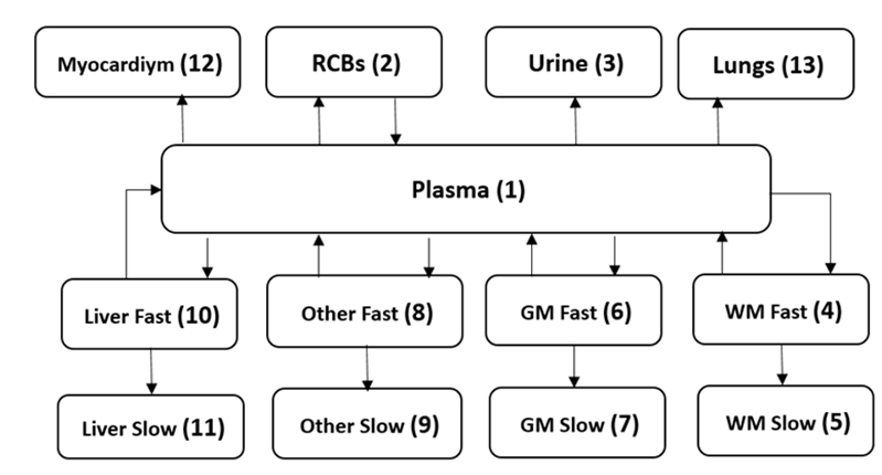
Figure 1.- 18F-FDG compartmental model described in described in (13) W. Li, D. Broggio, A. Giussani, T. Vrba, K. Hürkamp, A. Kamp, D. Noßke, L. Struelens, P. Covens: “EURADOS Intercomparison on Compartmental Model for 18F-FDG Developed by Hays and Segall”, Neuherberg, July 2021. DOI: 10.12768/zz8y-xw93. (https://eurados.sckcen.be/sites/eurados/files/uploads/Report-Publications/Reports/2021/EURADOS-Report-2021-04.pdf )
Input:
Solved with BIOKMOD SysModel2 package
Figure 2.- Time activity curves (TAC) for each compartment in function of the time (in min). Note: Due to we used 1 Bq in time t=0, it represent too the Fractional activity in each compartment.
◼
To compute the disintegrations acumultated and the Time Integrated Activity Coeffs. at (min): {0.1, 1, 10, 1000};
The OIR ICRP models
The OIR ICRP models
The ICRP models the human body divided in subsystems (Fig 3):
1
.The human respiratory tract model (HRTM), described in ICRP 130. When the intake occurs by inhalation although some parameters have different values depending on some characteristic of the aerosol’s intake (e.g. AMAD, vapor, chemical compositions, etc.).
2
.The human alimentary tract model (HATM), described in ICRP 100.
3
.Specific subsystems for the rest of compartments (“Systemic compartments”). The Systemic compartments are specific of each element. Although, sometimes, several elements form a group with the same biokinetic model (e. g. Lanthanides).
Fig 3.- Conceptual OIR ICRP Models.
The iodine model
Figure 4.- Iodine Model ICRP 137 (4).
A case of iodine 131 injection
A case of iodine 131 injection
Package OIRModels
BIOASSAY evaluation
BIOASSAY evaluation
Bioassays measurements can be used to estimate unknown intakes. BIOKMOD provides access to this kind of problem (http://oed.usal.es/webMathematica/Biokmod/ → Bioassay Evaluation). Bioassay data are fitted to the biokinetic model using the Maximum likelihood method or MLM (15)
Bioassays measurements can be used to estimate unknown intakes. BIOKMOD provides access to this kind of problem (http://oed.usal.es/webMathematica/Biokmod/ → Bioassay Evaluation).
As example, consider the following case: A person was exposed to the inhalation of an unknown intake of I131 in vapour form over three consecutive days. Three days after the last intake was measured the 131I content at the thyroid during three consecutive days: { di (day), mi (Bq), ui }: {{7, 2.1 10^4, 10^3}, {8, 2.5 10^4, 10^3}, {9, 1.5 10^4, 10^3}}.
Using the OIRModels package
Dose coefficients for I-131. ICRP Data Viewer (https://www.icrp.org/docs/ICRP%202022%20OIR%20Electronic%20Annex%20Distribution%20Set.zip)
Fitting models
Fitting models
Sometimes we may be interested in estimating a specific parameter of a model. This can be done by measuring the content in a specific compartment of the model or the urine or fecal excretion.
Suppose the simplified iodine model (Figure 5) where k12 and k23 transfer coefficients are unknown. Consider the case of a person who has been injected with I-131 and we want to calculate the rate of transfer from the thyroid gland.
There was no I-131 in the compartments at t= 0, so that the initial condition is: {0, 0, 0}. The objective is the estimation of coefficients k12 and k23. Figure 5 shows the input and results obtained using BIOKMOD.
Outputs
CITE THIS NOTEBOOK
CITE THIS NOTEBOOK
BIOKMOD: a web program to health physics and nuclear medicine application
by Guillermo Sánchez
Wolfram Community, STAFF PICKS, April 11, 2025
https://community.wolfram.com/groups/-/m/t/3443048
by Guillermo Sánchez
Wolfram Community, STAFF PICKS, April 11, 2025
https://community.wolfram.com/groups/-/m/t/3443048