The Wolfram Emerging Leaders Program: High School (WELP:HS) is a remote, semester-long program designed for exceptional graduates from the Wolfram High School Summer Research Program to continue to develop their skills. Students work in a small group over the course of a semester to do either a research-based project or a product development–based project under the guidance of expert mentors. Projects are centered around a topic at the intersection of the group’s interests.
In this project, we investigate deterministic graph-walk hashing, where each hash unit combines a graph structure and a traversal rule to map inputs into structured graph walks. Using various graph types, we test properties such as collision resistance and hash security, also known as the avalanche effect. Graph walking can meaningfully influence hash behavior, potentially displaying the concept’s feasibility for further exploration.
Introduction
Introduction
Hash functions are essential tools in computer science, serving roles in data integrity, encryption, and efficient information retrieval. Most traditional designs rely on arithmetic or bitwise transformations, while graph-based methods remain largely unexplored. This project introduces a structural approach to hashing that uses graph theory to produce environments for transforming input data.
Throughout the project, we refer to any particular hash function that converts a set of integers into a graph walk as a unit. Each of these units are composed of a graph and a traversal rule that uses an integer from input to dictate which edge to traverse. We have also quantified collision resistance and hash security, as described in the following sections. We will use these metrics to evaluate effectiveness of units whose graphs may be classified by a particular family.
Exploratory Behavior on Random Graphs
Exploratory Behavior on Random Graphs
To begin, we consider random walks on a randomly generated graph. We generate such a graph using the Erdős–Rényi model, constructed via a Bernoulli graph distribution on vertices with edge probability (Chatterjee, Varadhan; Krivelevich, Sudakov). In this model, each pair of vertices is connected independently with probability . To ensure the graph remains sparse, we choose to be sufficiently small, particularly with . With this choice, the expected degree of each vertex stays constant while the total number of edges grows linearly with , which is a standard result in random graph theory.
n
p
p
p
pO
1
n
n
Creates a Erdős–Rényi model graph
In[]:=
RandomGraph[BernoulliGraphDistribution[15,1/15],ImageSize->Large]
In[]:=
randomTestGraph=
;
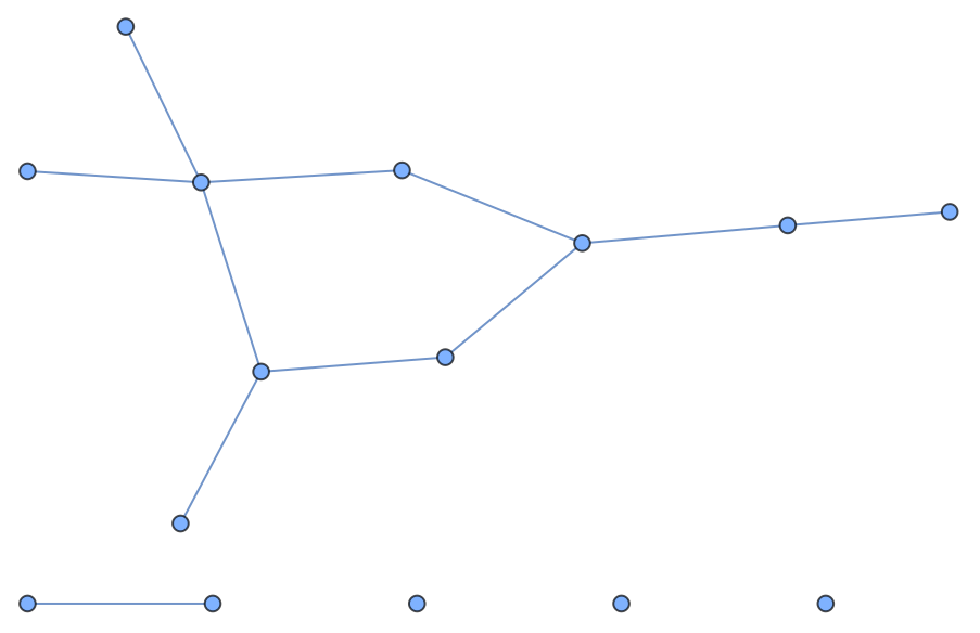
The randomness of the initial test graph is evaluated by visualizing the distribution of the number of edges incident to each vertex.
Bar Chart for numbers of edges each vertex has
BarChartTally[Table[Length[AdjacencyList[randomTestGraph,i]],{i,1,15}]][[All,2]],
Out[]=
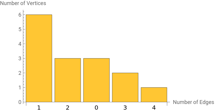
After generating a random test graph, the next objective is to evaluate how effectively the graph expands a walk. This is important for the intended application because stronger expansion leads to greater mixing in the resulting hash, which is desirable. To conduct this evaluation, a traversal rule must be established for how the walk progresses through the graph in order to measure how efficiently it spreads across vertices.
Movement Plan
Movement Plan
The walk begins at a predetermined starting vertex. At each step, one incident edge is selected using Wolfram’s pseudorandom number generator, and the walk proceeds along that edge. The walk terminates once a specified walk length, measured in the number of vertices visited, is reached. The walk length is defined as
, where is the number of vertices. By the Pigeonhole Principle, a perfectly spreading walk would require at least steps to visit all vertices, which corresponds to the existence of a Hamiltonian path. However, Hamiltonian paths are relatively rare in random graphs. To compensate for this and increase the likelihood of broader coverage, the walk length is scaled by a factor of two, providing a simple and effective method for promoting stronger mixing across the graph.
2n-1
n
n-1
Code that outputs the path for a random walk
In[]:=
randomWalkGraph[graph_,start_,steps_]:=Module[{current=start,path={start},neighbors},Do[neighbors=AdjacencyList[graph,current];current=Which[neighbors=={},current,True,RandomChoice[neighbors]];AppendTo[path,current],{steps}];Return[path]];
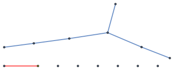
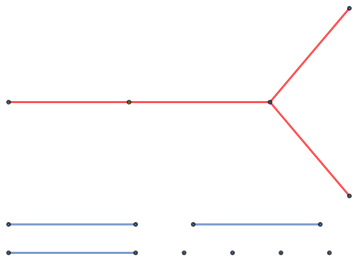
This visualization function accepts a graph and a corresponding walk on that graph, and highlights the path taken during the walk.
This visualization function accepts a graph and a corresponding walk on that graph, and highlights the path taken during the walk.
Code that takes in a path and outputs it on the graph
visualizePath[graph_,vertexPath_List]:=With[{edgePath=Table[UndirectedEdge[vertexPath[[i]],vertexPath[[i+1]]],{i,1,Length[vertexPath]-1}]},Return[HighlightGraph[Graph[graph,VertexSize->0.1],{Style[vertexPath[[1]],Yellow],Style[edgePath,Red]},ImageSize->Large]];]
A set of walks is generated on the random graph. While the walks appear random, they do not seem to effectively traverse the entire graph. This observation is examined further using additional data.
Code that generates the sparse Erdős–Rényi model graphs
In[]:=
testSet=Table[With[{graph=RandomGraph[BernoulliGraphDistribution[15,1/15]]},{graph,randomWalkGraph[graph,1,30]}],10];
In[]:=
Grid[Partition[Table[Graph[visualizePath[testSet[[i]][[1]],testSet[[i]][[2]]],ImageSize->Small],{i,1,8}],4],Dividers->All]
Out[]=

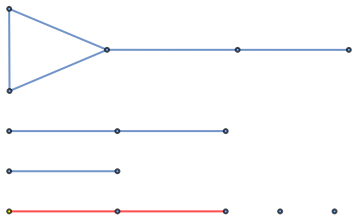

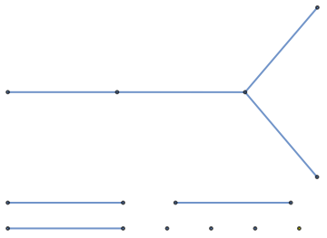

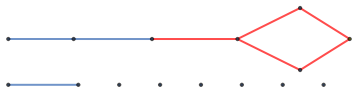
Testing
Testing
To expand the dataset and verify that these walks are not outliers, the process is repeated for every possible starting vertex across multiple randomly generated graphs. Although preliminary observations suggest that these graphs do not expand walks effectively, conclusions should not rely solely on visual evidence. To evaluate expansion, a simple metric is introduced: the ratio between the number of distinct vertices visited during the walk and the total number of vertices in the graph.
Under this metric, a perfectly expanded walk would visit all vertices at least once. In contrast, a poorly expanded walk would visit only two vertices, given that the walk consists of steps.
N
2N
Creates visualizations for the expansion quality of the graph based off all all starting points and pseudorandom next-vertex choices.
In[]:=
Grid[Partition[Module[{size=50,data},data=Table[Module[{graph=RandomGraph[BernoulliGraphDistribution[size,1/size]],walks},walks=Table[randomWalkGraph[graph,start,size*2-1],{start,1,size}];Length[DeleteDuplicates[#]]&/@walks],6];ListPlot[#,Epilog->{Red,Line[{{0,50},{Length[#],50}}],Text[Style["Optimal",Red,FontSize->Tiny],{Length[#]/2,52}]},PlotRange->{{0,size},{0,55}},AxesLabel->{"Starting Vertex","Expansion"},ImageSize->Medium]&/@data],3],Dividers->All]
Out[]=
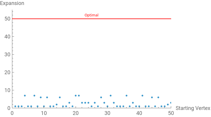
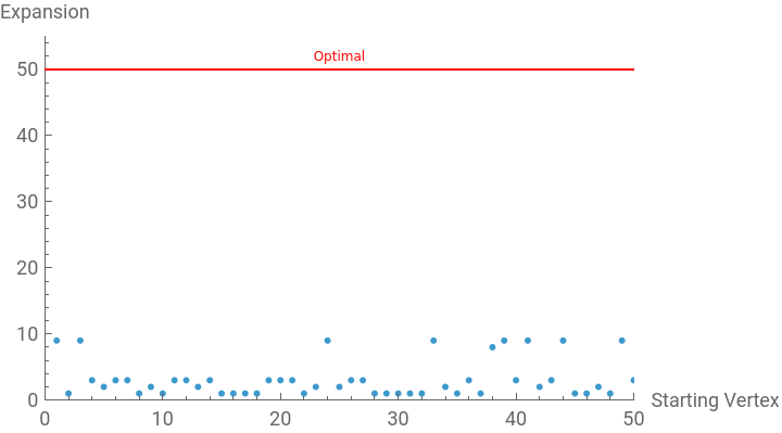
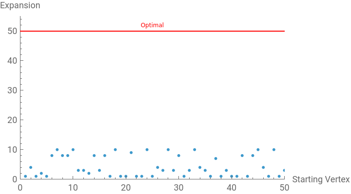
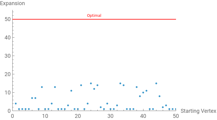
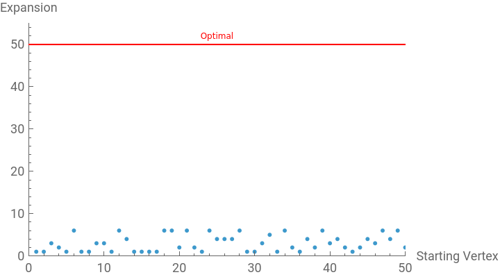
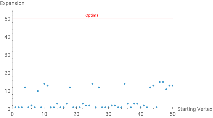
All data points lie significantly below the optimal expansion line. This indicates that randomness produces highly irregular degree distributions and weak expansion properties, limiting how effectively a walk can spread throughout the graph. Consequently, although the focus remains on sparse graphs, the analysis shifts away from unrestricted randomness toward constructions of deterministic traversal rules.
Defining Functions
Defining Functions
We now move from randomized exploration to deterministic construction. Rather than allowing randomness to dictate movement, we introduce a function that may be used to construct a unit as a defining function. In our exploration of defining functions, we first created a traversal rule that may be applied to a vertex of any graph. Notice that the list of neighbors and an input value are used by the traversal rule to understand the context in which it is being applied.
A simple example of a traversal rule is computing a quick modular arithmetic calculation using input value and the number of neighboring edges on the graph. Our implementation of such a traversal rule is shown below as the standardHash function.
Standard traversal rule that selects the next node using modular arithmetic computations
Similarly, we could use this modular arithmetic process after reordering our list of neighbors. For instance, we may use the degree of the neighbors themselves as a metric for sorting this list. Following this assortment, we may simply select the next node in the graph walk through our prior modular arithmetic calculation.
Traversal rule that selects the next node by sorting the neighbors by degree and applying modular arithmetic on the input value
Traversal rules are also often defined using bitwise operators, primarily the xor function. In this particular situation, two easily accessible constants are the current node and input value since they are both parameters for every traversal rule. We may apply Wolfram’s BitXor function and apply our modular arithmetic process on the result rather than the input value.
Traversal rule that applies modular arithmetic on the XOR output of the value and current node
Traversal rule that uses Knuth’s multiplicative constant and the bitwise AND function to identify the next node
Another widely recognized algorithm to deterministically select the next node in a traversal rule is to employ bit shifting. Between bit shifts, we may take an xor value with the original value to avoid redundancy between shifts. In order to maximize diffusion, as well as the avalanche effect, the bit shifting method that has been found to be the most effective is shifting 13 bits left, 17 bits right, and 5 bits left once again (Chen; Bentley, Sedgewick). To couple the input value with the current state of the graph, we apply our bit operations on the sum of these two quantities rather than either one individually, as shown below.
Traversal rule that uses bit shifts and XOR outputs to determine next node of graph walk
Since we have created a suite of traversal rule, we may now consider the other component of each unit, a graph, which can be created with built-in Wolfram functions, such as the sample graph shown below
Sample graph made with built-in Graph functionality
Combining these two components, we created a function that simulates units. For each integer in our input set, we may apply standardHash to move to the next node in the graph, appending to the end of the graph walk. For instance, consider an input of {3,1,4,1,5,9} for a unit that is composed of sampleGraph above and standardHash.
Sample input list that is used for future testing
We may simply run through all the values in the input set and apply our standardHash traversal rule, as shown in the code below.
Simulates the example unit made up of sampleGraph, sampleInput, and standardHash
We generalized this method for any unit to create the GraphWalkHash function shown below.
Function that uses a graph, traversal rule, and set of input integers to produce a graph walk
Testing the GraphWalkHash function with the original example unit provides the same graph walk as output, which is shown from the result below. In other words, if we use standardHash to encrypt sampleInput on sampleGraph, the resulting graph walk would indeed be {3,4,3,4,5,4}.
Produces graph walk with the example unit made up of sampleGraph, sampleInput, and standardHash
Quantifiable Metrics
Quantifiable Metrics
We define collision resistance as a metric that measures the probability for two different input sets in a hash function to produce two different outputs. Hence, collision resistance is a real number from 0 to 1, inclusive. In order to quantify this computationally, we can start by testing if the outputs under two inputs of a unit are identical, which can be done by checking equality on two different GraphWalkHash arguments.
Checks for equal results from GraphWalkHash
Additionally, to begin collecting empirical data on any given unit, we may begin randomizing the input lists to the equalResults function above. For simplicity, we may let each of these randomized lists be of length 10 and contain integers from 1 through 100, inclusive.
Checks output equality for a unit with two randomized input lists
Repeatedly calling the test function above and counting the proportion of results that are false would provide an empirical estimate of collision resistance for a given unit. In order to provide credibility for the accuracy of this estimate, we may also include simulations as a variable that dictates the number of times that the unit is tested for output equality.
Estimates collision resistance for a hash function unit
Estimates collision resistance with 100,000 simulations of the unit built with sampleGraph and standardHash
The result above suggests that, for the unit composed of sampleGraph and standardHash, while two different inputs produce distinct outputs, there are instances in which the same output may be produced by different inputs. In order words, it is possible to construct two lists of integers such that encrypting them with this unit produces the same graph walk.
We next define hash security as a metric that measures the expected proportion of the integers in the output graph walk that change when a random value in the input is altered. Hence, hash security is also a real number from 0 to 1, inclusive. We can start calculating this value by counting the proportion of values that are different between two equally sized graph walks.
Counts the proportion of values that are different in two equally sized graph walks
We can now derive the two walks that can be used as inputs for the walkDifference function above. One of these graph walks would be from an original input set, which can be derived from the GraphWalkHash function, and the other graph walk would be derived after a value of the input set is replaced. We will call this altered input set as a mutated input.
Measures the impact of a change in input list on the output of a given unit
We may repeatedly call this walkSensitivity function and calculate the average number of values in the encrypted graph walk that change to estimate hash security for a given unit. Similar to the function for collision resistance, we may also include simulations as a variable that dictates the number of times that walk sensitivity is calculated.
Estimates hash security for a hash function unit
Estimates hash security with 100,000 simulations of the unit built with sampleGraph and standardHash
The result above suggests that when a randomly chosen value of an input list is replaced, approximately 16.6% of the values in the output graph walk are altered. Although this change is significant, it does not imply an evident avalanche effect in the hash function unit.
Additional Measures
Additional Measures
The provided code contains two functions, BruteFindCollisions and BruteCollisionQ, which are designed to analyze hash collisions in a graph-based hashing scheme. Although these functions were ultimately not used in the final analysis, they serve an important role in evaluating the one-to-one requirement of a hash function by determining whether distinct input bit sequences can produce identical hash outputs.
◼
BruteFindCollisions: This function generates all possible input bit sequences for a specified number of bits, applies the hashing function to each sequence using the designated graph, and stores the results in an association. It detects collisions by identifying hash outputs that correspond to multiple input sequences and returns a formatted list displaying these collisions along with the number of inputs that produce each repeated output.
◼
BruteCollisionQ: This function determines whether any hash collisions exist by hashing each possible input bit sequence and comparing the results against previously computed hashes. The function immediately returns True upon detecting a collision; otherwise, it returns False after evaluating all input sequences.
Graph Types
Graph Types
Wolfram’s built in CayleyGraph function takes a PermutationGroup as an argument. The PermutationGroup takes a list of cycles as an argument. In order to format Cayley graphs in such a way that they are fairly easy to read and match with the input constraints of GraphWalkHash, we created the Cayley function below.
Produces cayley graphs from a list that defines a group of cycles
Produces a cayley graph with the Cayley function
The nodes of a Kneser graph are fixed length subsets of a set and edges are drawn between two nodes if and only if their corresponding subsets are disjoint. For instance, if we let the length of the set be n = 5 and the length of the subsets be k = 2, the graph would be as shown below.
Produces a Kneser graph with n=5 and k=2
However, to conform with the constraints on GraphWalkHash, we must adjust this slightly in generalization in order for the vertices to be represented by integers rather than lists. We may do so by drawing edges between the indices in the vertex list rather than between the elements of the vertex list themselves.
Kneser Graph Generator
Produces a Kneser graph with n=5, k=2, and integer vertices
Notice that the graph above is isomorphic to the graph previously produced, implying that the only difference between the two representations is the labeling of the vertices.
A Hypercube graph takes one input, n, to create an n-dimensional cube. For instance, Wolfram’s built-in HypercubeGraph function produces the results below.
Creates three hypercube graphs of different dimensions
In order to meet the criteria for our GraphWalkHash method and traversal rule, we reformat this built-in function as follows.
Reformatted version of HypercubeGraph function
Ramanujan Graphs
Ramanujan Graphs
Having explored standard graph types, we now turn to a mathematically sophisticated graph family, namely Ramanujan graphs. Ramanujan graphs are distinguished from the previously considered graphs by their specific construction methods, as we proceed to investigate.
Every Ramanujan graph is associated with a set of eigenvalues, which can be computed from its adjacency matrix. An eigenvalue measures how the matrix acts on certain special vectors, scaling them without changing their direction. In the context of graphs, these values encode global connectivity and interaction patterns between vertices (Chung).
Of particular interest is the second largest nontrivial eigenvalue, as it provides a measure of the graph’s expansion properties and the efficiency of mixing in a random walk. Smaller values indicate better expansion, meaning that walks spread more uniformly across the graph.
While a complete graph achieves maximal expansion, it is impractical for large graphs because the number of edges scales quadratically with the number of vertices. This growth can quickly exceed computational memory limits. For this reason, sparse graphs are preferred, as they maintain strong expansion properties while keeping the edge count manageable, allowing the construction and analysis of larger graphs.
To illustrate the computational challenges of dense graphs, consider the rapid growth in edge count for complete graphs as the number of vertices increases
Complete Graph Growth
As stated earlier, complete graphs achieve maximal expansion, but the quadratic scaling of edges limits practical usage for large graphs. Naturally, we proceed to consider sparse graphs that grow more slowly in edge count and remain manageable as the number of vertices increases. A representative example of a sparse graph is the Petersen graph, a subset of Kneser graphs, which maintains a relatively small size even as vertex count increases
Sparse Petersen Graphs
This property ensures optimal expansion while maintaining sparsity, making Ramanujan graphs ideal candidates for applications where both efficiency and strong mixing are important.
Explicit constructions of Ramanujan graphs exist, including Lubotzky–Phillips–Sarnak (LPS) constructions, probabilistic methods, and 2-lift techniques (Lubotzky, Phillips, Sarnak). For the purposes of this project, we do not implement these explicit constructions. Our focus remains on exploring parameter based graphs and traversal rules, which are more straightforward to generate and more adaptable for experimentation.
Random Regular Graph Generator
The examples below show random regular graphs with fixed degree and increasing numbers of vertices
Examples of Random Regular Graphs
Example of a disconnected regular graph
Although disconnected regular graphs are unlikely in randomized constructions, connectivity is essential for meaningful traversal. For completeness, a connectivity check is included when generating candidate graphs.
Random Graph Selection Algorithm
This algorithm repeatedly generates random regular graphs and computes the second largest eigenvalue in absolute value using the Arnoldi method (Huhtanen). At each iteration, the current graph is compared against the best candidate achieved so far, and the graph with the larger spectral gap is retained.
Random Near-Ramanujan Examples
Testing
Testing
We will evaluate these new graphs, which our construction and prior graph theory results indicate are likely to be better expanders while maintaining sparsity. The testing procedure will follow the same methodology used previously for poorly expanding random graphs.
Creates visualizations for the expansion quality of the graph based off all all starting points and pseudorandom next-vertex choices.
The results differ markedly from those observed with the previous graphs. The clusters lie much closer to the optimal expansion line, indicating that the function successfully generates graphs suitable for our intended applications.
Testing Traversal Rules with Graphs
Testing Traversal Rules with Graphs
In the following experiments, we restrict attention to the structured graph families introduced earlier, namely the Cayley graphs, Kneser graphs, and Hypercubes. Since Ramanujan graphs were explored in detail in the preceding section, they are omitted here to keep the focus on graph families with simpler constructions and more transparent combinatorial structure.
To set up our testing units, we begin by putting together a list of all our possible graphs and a list of our traversal rules.
Starting with our Cayley graphs, we propose four different variations to use for testing, namely the S3,S4,S5 symmetric groups as well as the D4 dihedral group
Four variations of Cayley graphs: S3, S4, S5, D4
Three variations of Kneser graphs: Petersen, (6,2), (7,3)
Finally, we will also test Hypercube Graphs in 3,4, and 5 dimensions
Three variations of Hypercube graphs
We may now create our graph and traversal rule lists.
Notice that every unit that we test is made up of a graph from graphList and a traversal rule from traversalList. Hence, we can measure collision resistance and hash security by simply selecting each pair and applying our respective functions.
Measures collision resistance for each hash function unit
Measures hash security for each hash function unit
We may display these results in the form of the tables below.
Recall that collision resistance values closer to 1.000 imply that the hash function almost never maps different inputs to the same graph walk.
Moreover, when a single flip in the input causes at least 50% of bits to flip, the hash function is considered to have effective hash security. Since we consider positive integers rather than bits, we can adjust this criteria to hash security values of at least 0.350 - 0.400.
Since most of the collision resistance values are extremely close to 1.000, we can begin filtering effective hash functions by hash security. In this fashion, we notice that the strongest individual results were
◼
Kneser(6,2) with xorHash: 0.403
◼
Kneser(7,3) with xorHash: 0.392
◼
Kneser(7,3) with xorShiftHash: 0.380
◼
Hypercube(5) with xorHash: 0.375
◼
Hypercube(5) with xorShiftHash: 0.372
Notice that each of these hash functions simulated a collision resistance of 1.000, ensuring that the hash function almost always maps different inputs to different graph walk outputs.
The series of simulations conducted above conveyed the following two takeaways
◼
xorHash was very effective
◼
Hash Security was typically greater than 0.2 for each tested graph
◼
Collision Resistance was at least 0.99996 for all tested graphs
◼
Kneser(6,2) and Kneser(7,3) were very effective
◼
Hash Security was greater than 0.2 for both graphs and all tested traversal rules
◼
Collision Resistance was at least 0.99999 for both graphs and all tested traversal rules
Multi-Graph Hash Function
Multi-Graph Hash Function
As an extension to the previously defined hash functions, we examined a production graph walks that were determined by a set of graphs rather than a singular graph
We start at vertex 1 of the first graph in the set and apply the traversal rule to determine the next vertex. We then “teleport” to the same-numbered vertex of the next graph. If no such vertex exists, we take a modular arithmetic calculation with this value and the number of vertices in this new graph. From here, we repeat this process until we have used every value in the input list, cycling through the set of graphs.
Since collision resistance values were extremely close to 1.000 in previous simulations, we would like to determine if using multiple graphs improves the hash security metrics.
We begin by creating a multi-graph equivalent for the previous GraphWalkHash function.
Returns a graph walk given a list of graphs, an input list, and a traversal rule
Along with this, we must create similar functions to calculate the hash security metric. In order to better interpret the produced hash security values, we slightly redefine the concept as follows. Rather than measuring the proportion of total values in the output that change under input change, we can measure the proportion of values after the index where the input change occurs. The new functions to calculate this are as shown below.
Returns a count of the number of different respective values between two list
Building off of this function, we measure our redefined hash security for a single multi-graph hashing simulation
Quantifies the impact of an input value on the following output values
Running MultiWalkSensitivity over multiple simulations with random input lists averages out to an accurate approximation of the hash security for a given hash function. We perform exactly this with the MultiHashSecurity function below.
Runs multiple simulations of MultiWalkSensitivty and returns the average as an approximation for hash security
Now that we have functions to can both simulate hash functions, produce graph walks, and calculate hash security, we may begin to perform simulations in a similar fashion to the single graphs previously. However, since performing a sufficient number of simulations over every non empty subset of our 10 graphs would have a large runtime, we instead take subsets for each category of graphs, namely Cayley, Kneser, and Hypercube.
We begin by creating an association for each of these graph categories so that the results display the name of the graph rather than the graph itself.
Associations for the three major graph categories
We may now take all non empty subsets of the keys of these three associations to obtain all subsets that we aim to simulate with. Recall that the built-in Rest function removes the empty set from a list.
All non empty subsets of graphs for the three major graph categories
For each of the subsets of the three graph categories, we simulate with the two traversal rules that proved to be most effective for single graphs, namely xorHash and xorShiftHash. For all six combinations of graph category and traversal rule, we run 100,000 simulations per subset.
Results from 100,000 simulations for each subset of graphs with both xorHash and xorShiftHash
Finally, recall that Kneser(6,2), Kneser(7,3), and Hypercube(5) proved to be effective in the single graph simulations. Here, we run simulations of both this set of three graphs, as well as the set of all ten graphs.
Results from 100,000 simulations of effective single graphs with both effective traversal rules
Results from 100,000 simulations of all ten graphs with both effective traversal rules
The following configurations achieved hash security values greater than 0.7
◼
Kneser(6,2) with xorHash: 0.757
◼
Hypercube(5) with xorHash: 0.753
◼
Hypercube(5) with xorShiftHash: 0.748
◼
Kneser(6,2), Kneser(7,3), Hypercube(5) with xorHash: 0.727
◼
Kneser(7,3) with xorHash: 0.722
◼
Kneser(7,3) with xorShiftHash: 0.717
◼
Hypercube(4), Hypercube(5) with xorHash: 0.716
◼
Hypercube(4), Hypercube(5) with xorShiftHash: 0.709
In nearly all cases, the higher hash security values were achieved by single graphs, particularly Kneser(6,2), Kneser(7,3), or Hypercube(5) paired with XOR based traversal rules, rather than multi-graph hash functions. These results indicate that hash security is dominated by the structural properties of individual graphs rather than alternating between multiple graphs.
We conjecture that this behavior arises from the multi-graph hashing procedure itself. Although each traversal step is computed within a single graph, the subsequent “teleportation” to a different graph disrupts the local structure on which the traversal rule may depend. This prevents the walk from evolving within one graph over many steps.
By contrast, a single highly structured graph allows deterministic traversal rules to repeatedly interact with the same patterns, potentially amplifying hash security, and maybe even collision resistance, across the entire walk, making these metrics a matter of depth over breadth.
Mixed Radix Stream Walks
Mixed Radix Stream Walks
We implement a mixed radix stream–inspired hash as a deterministic graph walk driven by integer interval splitting. Starting from a fixed vertex, the input bitstring is interpreted as an integer and mapped to successive vertices by partitioning the current integer range according to the degree of the current vertex. At each step, a splitting function selects the next vertex using the Floor operation, updating the interval and advancing the walk. The traversal is performed for a fixed number of steps, and the resulting walk constitutes the hash output.
Integer-Based Mixed Radix Graph Walk Hash
The splitting function determines which neighboring vertex is selected at each step of the walk. It partitions the current integer interval into equal subranges and uses the input value to select the corresponding partition, returning both the chosen index and the updated bounds for the next iteration.
Integer Interval Splitting Function
This function serves as the core interval-selection mechanism for the mixed radix hash, translating integer input values into deterministic traversal decisions.
We now generate a random 6-regular graph as a default input for the mixed radix hash functions.
Default Random 6-Regular Graph
We can now apply the mixed radix stream hash function to generate a traversal on the default graph using a sample input bitstring. This demonstrates how the integer-based splitting function produces a deterministic walk.
Example Graph Walk Using Mixed Radix Hash
We define a function to visually highlight the vertices and edges traversed during a mixed radix graph walk. This allows us to inspect paths and identify frequently visited nodes.
Graph Walk Highlight Function
Highlighting a Single Walk
Vertices visited and the connecting edges are highlighted in red, illustrating the path induced by the input. For instance, we can track the most frequently visited vertices for a large number of random inputs to identify where mixed radix stream hash functions may face traffic.
Most Frequently Visited Vertices Over 10,000 Random Inputs
The highlighted walks demonstrate that vertices are well-dispersed throughout the graph. Walks do not repeatedly traverse only a small subset of nodes, which is critical for ensuring collision resistance and overall hash security.
Average Collision Resistance over Unique Walks
Distribution of Collision Resistance for Walk Occurrences
This exhaustive test indicates that there are no collisions among all 1,048,576 inputs, suggesting that the mixed radix walk provides a strong foundation for a hashing scheme.
To fully meet hash functions requirements, we finally convert the graph walk into a binary hash of uniform length. The hashify function below encodes each vertex in the walk as a fixed-length binary number, ensuring that the resulting hash is consistent in size regardless of the input.
Hashify Function for Uniform Binary Output
Below are three examples of this hashify method put to use.
Hashify method applied on the bit string 110010110001011
Hashify method applied on the bit string 1101
Hashify method applied on the bit string 1
We observe that inputs of different lengths produce hash values that are well-dispersed, making it difficult to infer the original input length from the hash alone, which is an important property for hash security.
We next examine how the hash distributes 1s across bit positions for a large set of random inputs. This analysis helps determine how uniformly the hash function uses each bit and whether any positions remain unused. The following code generates 10,000 random 10-bit inputs, applies the mixed radix hash, and counts the number of 1s in each bit position.
Counting 1s per Bit Position Over 10,000 Random Inputs
Analysis shows that most bit positions have thousands of occurrences of 1, while a few remain 0.
Dividing these counts by 10,000 produces the average frequency of 1s per bit position, displayed in the graph below. The resulting pattern exhibits many ups and downs, indicating irregularity across positions. This variation improves diffusion and ensures that hash outputs differ substantially between inputs, enhancing security.
To assess the typical density of 1s in the hash outputs, we calculate the overall average value across all bit positions to be 0.391371.
Although one might expect this average to be around 0.5 for a uniform distribution, the observed value is 0.39. This deviation is likely influenced by the specific structure of the graph used. To determine whether the low average value observed previously is an artifact of a single graph or a general feature across mixed radix hash functions, we repeat the analysis using 100 different random graphs. This provides a more rigorous study of the hash function’s structure and reduces the impact of confounding variables within the graph itself.
Average of all Bit Values Across 100 Random Graphs
The resulting average of 0.38 is similar to the 0.39 observed with a single graph, suggesting that the prevalence of 0s is inherent to the design of the hash function rather than a property of any particular graph.
To further examine the distribution across positions, we plot the mean value of each bit over 100 random graphs.
Visualization of Bit Position Averages
The plot shows that most positions remain below 0.5, with occasional drops at certain positions that also appeared in the single-graph analysis. This suggests that the bias toward 0s arises from the structure of the mixed radix stream hashing algorithm itself, likely due to the way integer intervals are partitioned and rounded with the Floor function, which systematically favors lower-indexed vertices in early steps of the walk.
While the hash function exhibits predictable bias toward 0s, it provides a foundation for refinement, for example by adjusting the interval-splitting scheme or varying vertex labeling to achieve better balance and more uniform bit distributions across positions.
Development on Traversal Rules
Development on Traversal Rules
This section provides a deeper analysis of traversal rules, independent of the process of encoding a walk into a cryptographic hash. Building upon earlier exploratory constructions, the emphasis shifts toward evaluating more structured traversal strategies and their impact on mixing behavior, collision resistance, and overall hash performance.
Reading Bit Strings by Sections
Reading Bit Strings by Sections
We begin by examining how the input should be interpreted during traversal. One natural approach is to read the input one bit at a time and use each bit value to determine which neighboring vertex to move to. Under this rule, a bit value of 0 or 1 selects between two available neighboring vertices.
Since this rule requires exactly two available traversal choices while excluding the previous vertex, it may only be consistently implemented on 3-regular graphs.
Creates visualizations of graph covering data
However, for this application, 3-regular graphs are not ideal. They provide relatively low entropy per step. Even if expansion were reasonable, graphs with larger degree would allow far more variability in traversal choices. Increasing the degree allows more information from the input to influence each step of the walk. To achieve this, the input must be processed in groups of bits rather than individual bits.
The traversal rule is described by the following pseudocode:
The resulting traversal procedure is implemented in the BitChunkWalk function below.
Creates random list of bits with a specified length
BitChunkWalk function as described above
We proceed to test this function with an effective random graph.
Outputs the walk path along with its visualization
One advantage of this traversal rule is that it produces behavior that is effectively random when the input is random. It also prevents immediate backtracking and tends to distribute the walk broadly across the graph. However, the rule does not provide strong security guarantees and lacks internal memory. Each step depends only on the current vertex, meaning that the traversal is determined locally and incorporates no additional information about the prior history of the walk beyond the current position. This limitation motivates the introduction of a state component to incorporate historical information into future traversal decisions.
Rolling State Graph Walking
Rolling State Graph Walking
To incorporate additional memory into the traversal, a state variable is introduced. This state uses the numerical labels of visited vertices and updates through specified arithmetic operations. Incorporating such memory is expected to reduce the likelihood of the walk becoming trapped in short cycles, since the evolving state can alter subsequent movement decisions. This addition may also improve security and increase variability in traversal behavior.
The code for the rollingStateWalk as described above
Outputs the walk path along with its visualization
The addition of the state, which introduces an extra step between standard moves, produces significantly greater movement and wider coverage in the walk. A potential risk exists if the state repeats itself multiple times due to the modular arithmetic, which could compromise the structure of the traversal.
Sponge Construction
Sponge Construction
Motivation for Sponge Construction
Motivation for Sponge Construction
It is a known result that a deterministic graph walk by itself is not a meaningful cryptographic hash function. This is because if the internal state consists only of a vertex v∈V(G), then the state space is small, the state evolution is fully observable, and the entire process can be backtracked easily. There is no hidden component of the state, so an observer who sees the walk can reconstruct prior states and potentially engineer collisions. Without additional structure, such a walk lacks the unpredictability and resistance properties required of a cryptographic hash.
Quick intro to the sponge construction
Quick intro to the sponge construction
Translating sponge concepts to graph walks
Translating sponge concepts to graph walks
Data Collection for Walk Collisions
Data Collection for Walk Collisions
The provided code includes two functions, BruteFindCollisions and BruteCollisionQ, designed to analyze hash collisions in a graph-based hashing scheme. These functions are essential for evaluating the one-one requirement of a hash function by determining whether different input bit sequences can produce the same hash output.
• BruteFindCollisions: This function generates all possible input bit sequences for a specified number of bits, hashes each sequence using the given function and graph, and collects the results in an association. It identifies collisions by checking for hash outputs associated with multiple input sequences and returns a formatted list showing these collisions along with the number of inputs that produce the same output.
• BruteCollisionQ: This function checks for the existence of any hash collisions by hashing each possible input bit sequence and comparing the results to previously seen hashes. It instantly returns True if it detects a collision, otherwise it returns False after examining all sequences.
Goes through all possible numbers up to some number of bits, searching for and outputting all collisions
Goes through all possible numbers up to some number of bits, returning whether there is a collision or not
Acknowledgements
Acknowledgements
We would like to thank Bertie Bennett for serving as our mentor on this project. His guidance, insight, and feedback were helpful throughout our research. We are also grateful to Rory Foulger for directing WELP and giving us the opportunity to explore such an engaging topic, as well as for his continued support, constructive feedback, and the time he dedicated to meeting with us to discuss our progress and essay writing.
Sources
Sources
◼
Chatterjee S and Varadhan SRS. The large deviation principle for the Erdős–Rényi random graph, 2011
◼
Krivelevich M and Sudakov B. The phase transition in random graphs – a simple proof, 2012
◼
Bentley J and Sedgewick R. Programming Pearls, 1986
◼
Chen P et al., Analysis of Hash Functions, 2007
◼
Chung F. A Generalized Alon‑Boppana Bound and Weak Ramanujan Graphs, 2016
◼
Huhtanen M. Arnoldi methods for the eigenvalue problem, 2012
◼
Lubotzky A, Phillips R, and Sarnak P. Ramanujan conjecture and explicit constructions of expanders, 1986
CITE THIS NOTEBOOK
CITE THIS NOTEBOOK
Hash functions from deterministic graph walks
by Girish Prasad, Alex Archerman, and James Badishkanian
Wolfram Community, STAFF PICKS, February 11, 2026
https://community.wolfram.com/groups/-/m/t/3638617
by Girish Prasad, Alex Archerman, and James Badishkanian
Wolfram Community, STAFF PICKS, February 11, 2026
https://community.wolfram.com/groups/-/m/t/3638617