This is a re-working and extension of a quadratic iteration visualization generated by Simon Tyler here.
Iterative Quadratic
Iterative Quadratic
Take a monic quadratic, :
:=+z+0,∈
2
z
ω
1
ω
2
ω
1,2
Generate random complex coefficients using :
ω
1,2
In[]:=
ω12:=RandomComplex[{-1-I,1+I},2]
Find the roots of and randomly shuffle these back in as = or = as the coefficients of the quadratic using to select the order:
r
1,2
ω
1,2
r
1,2
ω
1,2
r
2,1
In[]:=
[ω_]:=SolveValues[+{z,1}.RandomSample[ω]==0,z]
2
z
Symbolic check:
In[]:=
Table[[{a,b}],4]//Grid
Out[]=
1 2 -4a+ 2 b | 1 2 -4a+ 2 b |
1 2 -4a+ 2 b | 1 2 -4a+ 2 b |
1 2 2 a | 1 2 2 a |
1 2 -4a+ 2 b | 1 2 -4a+ 2 b |
Repeat times using :
n
In[]:=
quadraticroots[n_]:=NestList[,ω12,n]
Estimate the maximum absolute value of the resulting roots:
In[]:=
quadraticroots[]//Abs//Max
4
10
Out[]=
2.21346
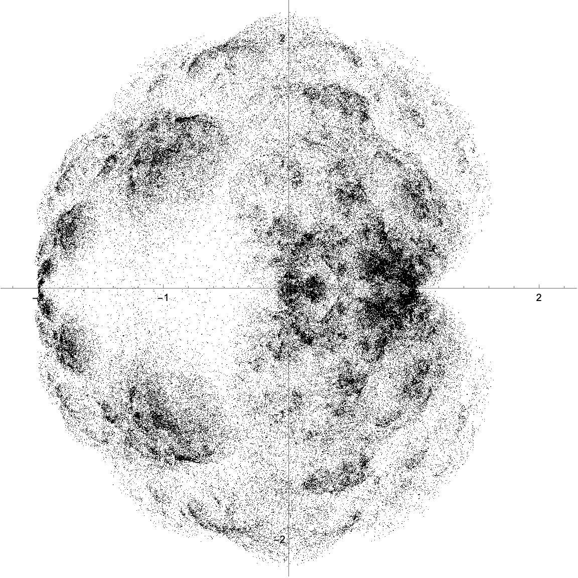
Produce an Argand plot of the generated roots:
In[]:=
Graphics{AbsolutePointSize[1],quadraticroots[]/.Complex[a_,b_]:>Point[{a,b}]},
5
10
Out[]=
Random Cubic
Random Cubic
Generalize the above code to a monic cubic, :
:=++z+0,∈
3
z
ω
1
2
z
ω
2
ω
3
ω
1,2,3
Generate random complex coefficients using :
ω
1,2,3
In[]:=
ω123=RandomComplex[{-1-I,1+I},3]
Out[]=
{0.165623-0.286416,-0.423783+0.0984421,0.220354+0.0448621}
Find the roots of and randomly shuffle these back in as the coefficients of the cubic using to select the order:
r
1,2,3
In[]:=
[ω_]:=SolveValues[+{,z,1}.RandomSample[ω]==0,z]
3
z
2
z
Repeat times using :
n
In[]:=
cubicroots[n_]:=NestList[,ω123,n]
Estimate the maximum absolute value of the resulting roots:
In[]:=
cubicroots[]//Abs//Max
4
10
Out[]=
2.88092
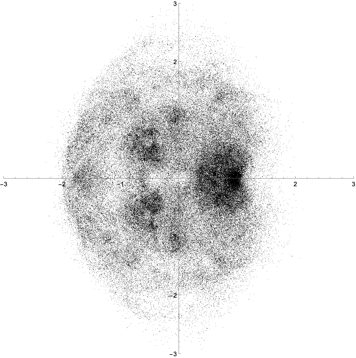
Produce an Argand plot of the generated roots:
In[]:=
Graphics{AbsolutePointSize[1],cubicroots[5]/.Complex[a_,b_]:>Point[{a,b}]},
4
10
Out[]=
Swapping r1↔r3
Swapping ↔
r
1
r
3
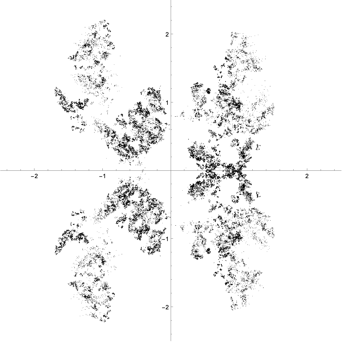
Again find the roots of but, instead of randomly permuting them, just randomly swap ↔ using and them put them back in as the coefficients of the cubic:
r
1,2,3
r
1
r
3
In[]:=
[ω_]:=SolveValues[+{,z,1}.RandomChoice[{Identity,Reverse}][ω]==0,z]
3
z
2
z
Repeat times using :
n
In[]:=
swappedroots[n_]:=NestList[,ω123,n]
Estimate the maximum absolute value of the resulting roots:
In[]:=
swappedroots[]//Abs//Max
4
10
Out[]=
2.49918
Produce an Argand plot of the generated roots:
In[]:=
Graphics{AbsolutePointSize[1],swappedroots[5]/.Complex[a_,b_]:>Point[{a,b}]},
4
10
Out[]=
CITE THIS NOTEBOOK
CITE THIS NOTEBOOK
Visualisation of iterated random complex roots
by Paul Abbott
Wolfram Community, STAFF PICKS, January 7, 2025
https://community.wolfram.com/groups/-/m/t/3351787
by Paul Abbott
Wolfram Community, STAFF PICKS, January 7, 2025
https://community.wolfram.com/groups/-/m/t/3351787