ABSTRACT (original article): This research-oriented report analyzes the impact of a class of time-independent forces and their time-dependent counterparts on the characteristics of solutions to the wave equation on a one-dimensional string. The solution of these equations, subject to Initial and Boundary Value (IBV) conditions, is investigated, yielding modified standing waves. Analyses are heavily Computer Algebra oriented. The popular Computer Algebra System (CAS), specifically Mathematica, has been pivotal in uncovering the numerical, algebraic, and graphical aspects of the investigation. The time-dependent force functions not only generalize the scope of the analysis but also possess 1) a character that their functionality by transitioning to the coordinate-dependent only is conducive to expected output, and 2) the absence of these forces frees the imposed IBV, conducive to the characteristics of the standard standing waves. This comprehensive report embodies an atlas of graphs for both mentioned forces. It is shown that the proposed one-dimensional time-independent forces give rise to previously unseen standing waves with a peculiar character. The report includes the essential Mathematica code for most calculations and all the graphs depicted. The report allows reproduction by individuals familiar with Mathematica. It is crafted and developed so that modification and generalization of the applied IBVs is readily possible. The Conclusion segment embodies a suggestion to expand the scope of future investigations. CITATION (original article): Sarafian, H. (2026) One-Dimensional Forced Standing Waves. American Journal of Computational Mathematics, 16, 1-13. https://doi.org/10.4236/ajcm.2026.161001
Keywords: Forced Standing Waves, Time-independent and dependent forces, Inhomogeneous Wave Equations, Computer Algebra System, Mathematica
1. Introduction
1. Introduction
The standard one dimensional elliptic homogeneous partial differential wave equation with constant coefficients is:
2
∂
∂
2
x
1
2
c
2
∂
∂
2
t
(
1
)with initial conditions;
u(x,0)=f(x) |
∂ ∂t |
(
2
)Equation (1) which has no boundaries describes the motion of an infinite long string with given initial conditions. Its solution bares the name of the excavator, D’Alambert [1] given in (3),
u(x,t)=[f(x-ct)+f(x+ct)]+g(ξ)ξ,
1
2
1
2c
x+ct
∫
x-ct
(
3
)The non-dispersive solution given in (3) is interpreted as moving waves in opposite direction. The is the speed of the non-dispersive waves.
c
The solution (3) and its applications are subject to analyses in physics and math courses.
One of the objectives of this report is to generalize (1), propose examples with solutions in the domain . Where ℓ is the finite length of the string.
The foremost generalization of (1) entails adding a variable term to convert the homogeneous in an in-homogeneous equation. The secondary aim stems from the fact that because of the restricted coordinate domain the traveling waves are reflected at the boundaries, potentially interfere forming so-called “stationary standing” waves. Addressing the impact of the non-homogeneous term on the characteristics of the standing waves concludes the report.
0≤x≤ℓ
The foremost generalization of (1) entails adding a variable term to convert the homogeneous in an in-homogeneous equation. The secondary aim stems from the fact that because of the restricted coordinate domain the traveling waves are reflected at the boundaries, potentially interfere forming so-called “stationary standing” waves. Addressing the impact of the non-homogeneous term on the characteristics of the standing waves concludes the report.
The generalized (1) is (4). The non-homogeneous term,, thereafter is called “Force,” bares the title of the article.
F(x,t)
2
∂
∂
2
x
1
2
c
2
∂
∂
2
t
0≤x≤ℓ
(
4
)Although different type boundary conditions may be considered, the interest is the one that the string of length ℓ is pined at both ends. This restricts the solutions of (4) satisfying,
u(0,t)=u(ℓ,t)=0,for
t > 0
(
5
)Compatible with (5) the string’s initial shape can be controlled via the initial conditions,
u(x,0)=f(x),
(
6
)And for the sake of argument and transparency of the calculation we consider the case that initially the string starts off freely, with no initial speed, i.e.,
∂
∂t
(
7
)In addition, two general cases are considered. 1a) is time-independent i.e. , and 1b) is coordinate and time-dependent separable function , i.e. .
With these assumptions in Section 2, solution of (4) is presented.
F(x,t)
F(x,t)=f(x)
F(x,t)
F(x,t)=f(x)g(t)
With these assumptions in Section 2, solution of (4) is presented.
This report composed of three sections. In addition to Sect 1, Introduction, Sect 2, is the Formulation and codes and embodies variety of graphic atlas. Conclusions are remarks are in Sect 3.
2a. Formulation and Coding
2a. Formulation and Coding
By applying the “modified” Fourier series with finite number of terms that controls the accuracy of the computation the formal solution of (4) is,
u(x,t)=(t)Sinx,
∞
Σ
n=1
u
n
nπ
ℓ
(
8
)The Fourier series with sine bases compatible with the the boundary conditions is called “modified” because it has time-dependent coefficients.
In aforementioned case Ia, ; the Fourier series expansion of the latter function is,
F(x,t)=f(x)
f(x)=Sinx,
∞
Σ
n=1
f
n
nπ
ℓ
(
9
)Comparing (8) and (9) shows the difference between the two mentioned series.
The orthogonality of the bases is,
ℓ
∫
0
nπ
ℓ
mπ
ℓ
0, | n≠m |
ℓ 2 | n=m |
(
10
)Utilizing (10) yields the constant coefficients of (9),
f
n
2
ℓ
ℓ
∫
0
nπ
ℓ
(
11
)Inserting (8) and (9) in (4) gives,
n=∞
∑
n=1
..
u
n
2
nπc
ℓ
u
n
f
n
nπ
ℓ
(
12
)Double super dot is the derivative with respect to time, concluding, each coefficient of ought to satisfy the ODE (13).
Sinx
nπ
ℓ
..
u
n
2
nπc
ℓ
u
n
f
n
(
13
)Equation (13) with a constant inhomogeneous term is a standard ODE, its solution is available e.g. [2][3][4],
u
n
f
n
ℓ
nπc
t
∫
0
nπc
ℓ
(
14
)Inserting (14) in (8) formally concludes the formulation segment of the report.
Because we are interested in the “forced” issue, , in (11) calls for some calculation. Quantity in (11) addresses the force and it can be any physically meaningful function. In our previous published article [3] we consider a class of polynomials. For the sake of consistency here we utilize the same; i.e. for . These functions my be replaced with functions of choice. From this point on we utilize a CAS, Mathematica [4] to carry out the symbolic calculations. Codes are given for reproduction and potential generalization.
f
n
f(ξ)
f(ξ)=
m
ξ
m=1,2,3,and4
2b. Descriptive Codes:
2b. Descriptive Codes:
Case I. , For the sake of simplicity the string length and the wave speed is set to unity. In the follow-up cases the time-dependent functions are parametrized via variable quantity α. All these quantities are stored in the values(1,2) lists,
F(x,t)=f(x)=
m
x
m=1,2,3and4.
In[]:=
values:={ℓ->1.,c->1.,α->0.}
In[]:=
values1:={ℓ->1.,c->1.,α->0.5}
In[]:=
values2:={ℓ->1.,c->1.,α->10.}
There is a one-to-one connection between the numbered equations and the codes. For instant the corresponding code of equation (11) is,
In[]:=
f1[n_,m_]:=Sinxx//Simplify
2
ℓ
ℓ
∫
0
m
x
nπ
ℓ
The is the power of the polynomiaI. For the is tabulated,
m
m=1,2,3and4
f1
In[]:=
tab1m=Table[{m,,f1[n,m]},{m,1,4,1}]
m
x
Out[]=
1,x,,2,,,3,,-,4,,
2ℓ(-nπCos[nπ]+Sin[nπ])
2
n
2
π
2
x
2(-2+(2-)Cos[nπ]+2nπSin[nπ])
2
ℓ
2
n
2
π
3
n
3
π
3
x
2(nπ(-6+)Cos[nπ]-3(-2+)Sin[nπ])
3
ℓ
2
n
2
π
2
n
2
π
4
n
4
π
4
x
2(24-(24-12+)Cos[nπ]+4nπ(-6+)Sin[nπ])
4
ℓ
2
n
2
π
4
n
4
π
2
n
2
π
5
n
5
π
Then (14) is coded,
In[]:=
u1[t_,n_]=Tabletab1mm,3Sinτ,{m,1,4};
ℓ
nπc
t
∫
0
nπc(t-τ)
ℓ
For instant, its element is,
rd
3
In[]:=
u1[t,n]〚3〛
Out[]=
-
2ℓ-ℓCos(nπ(-6+)Cos[nπ]-3(-2+)Sin[nπ])
4
ℓ
cnπt
ℓ
2
n
2
π
2
n
2
π
2
c
6
n
6
π
Equation (8) for the sum of the first 5-terms is,
In[]:=
u1Sum[x_,t_]=Tablem,Sumu1[t,n]mSinx/.values,{n,1,5},{m,1,4};
2
ℓ
nπc
nπc
ℓ
It’s first term corresponding to is,
1
x
In[]:=
u1Sum[x,t]〚1,2〛;(*theoutputissuppressed*)
The coefficients of the first five terms are;
In[]:=
{u1Sum[x,t]〚1,2,1,1〛,u1Sum[x,t]〚1,2,2,1〛,u1Sum[x,t]〚1,2,3,1〛,u1Sum[x,t]〚1,2,4,1〛,u1Sum[x,t]〚1,2,5,1〛}
Out[]=
{0.020532,-0.00128325,0.000253481,-0.000080203,0.0000328511}
This shows the coefficients alternate in sign and descending drastically. The latter justifies the series is converging and five terms in (8) is adequate.
Indexing the terms yields additional information. The outputs are suppressed but one
In[]:=
{u1Sum[x,t]〚1,2,2〛,u1Sum[x,t]〚1,2,2,1〛};
In[]:=
{u1Sum[x,t]〚1,2,3〛,u1Sum[x,t]〚1,2,3,1〛};
In[]:=
{u1Sum[x,t]〚1,2,4〛,u1Sum[x,t]〚1,2,4,1〛}
Out[]=
{-0.000080203(1.-1.Cos[12.5664t])Sin[12.5664x],-0.000080203}
In[]:=
{u1Sum[x,t]〚1,2,5〛,u1Sum[x,t]〚1,2,5,1〛};
For instance within the desired time span the graph of each mode can be animated, e.g. the mode associated with the 4th polynomial is,
In[]:=
Manipulate[Plot[Evaluate[u1Sum[x,t]〚1,2,4〛],{x,0,1},PlotRange{-0.0002,0.0002},GridLinesAutomatic,AxesLabel{"t","4th term"},PlotLabel"α=0"],{t,0.1,3.99,0.01},SaveDefinitionsTrue]
Out[]=


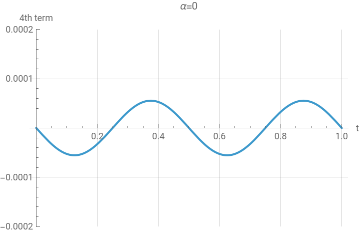
Finally, the animation of the collective modes corresponding to the individual polynomial is shown in Fig 1.
Figure 1. Profile of the vibrating string associated to the individual polynomial.
Animation of the profiled vibrations shows the string always keeps its positive amplitude, it never crosses the horizontal axis. This feature distinguishes itself from the classic standing waves.
Additional useful detailed codes for interested individual are. Outputs are suppressed.
The code for (11) is,
its tabular elements are,
The code associated with (14) is,
For instant, its 4th element is,
Equation (8) for the sum of the first five terms is,
Tabulated numeric coefficients of the terms of this sum are,
Table 1. Accuracy of the two different codes.
Within the desired time span the graph of each mode can be animated. For instance mode associated with the 1st element of the polynomial is,
Figure 2. Animation profile of the standing wave associated with the 1st element of the polynomial.
The animation reveals that the amplitude always stays positive, never crosses the horizontal axis.
E.g. its fourth term is,
Table 2. This table compares the coefficients of the terms in the Sum. The The description of this table is the same to table 1.
As shown the both coefficients are consistent alternating in signs and progressively diminishing in values.
Similar to Fig 3, each mode can be animated. The associated code is, however the individual output is suppressed.
An atlas of the general animation is formed,
Figure 4. Similar description as Fig 3.
The impact of the time-dependent component of the applied force is evedent. The animation shows the amplitude becomes negative, it cross the horizontal axis.
The previous code associated to (8) is modified,
Sample of its indexed term leading to the numeric coefficients are tabulated.
Table 3. Description is the same as Table 2. A comprehensive numeric table of the coefficients for the three studied cases.
Table 3.
The general feature of Table 3 is self explanatory. E.g. the coefficients irrespective to the case of interest have alternative signs. Their numeric values drastically decreasing signifying the convergence of the series at hand.
Figure 5. Description is similar to Fig 4.
Figure 6. Impact of the time-independent forces on early stage of the vibrating string.
Noticing, the amplitudes are very small. Nonetheless this shows different forces have distinct distinguishing effects.
Conclusions and Remarks
Conclusions and Remarks
D’Lambert waves subject to the solution of the unrestricted partial differential equation with constant coefficients has been modified by considering a finite length string subject to external forces. Two different class of forces, time-independent and time-dependent are considered subjected to certain boundary restrictions. Most of the calculations are carried out utilizing a CAS, Mathematica. Codes are provided for reproduction. An atlas of the graphs for better understanding are provided. This report deviates from traditional reports because it does not just gives the formulation, it embodies numeric and graphics coded results.
Interested readers may find [5][6] resourceful for Mathematica coding.
Interested readers may find [5][6] resourceful for Mathematica coding.
Conflict of Interest
Conflict of Interest
The author declares no conflicts of interest regarding the publication of this paper.
References
References
[1] Farlow, S.J. (1982) Partial Differential Equations for Scientists and Engineers, Dover Publications, Inc, New York.
[2] Gockenbach, M.S. (2011) Partial Differential Equations, Siam, Philadelphia.
[3] Tenenbaum, M., Polland H. (1963) Ordinary Differential Equations, Dover Publications, Inc., New York.
[4] Rainville, E.D. (1964) Elementary Differential Equations, The Macmillan Company, New York.
[4] Wolfram, S. (2003) The Mathematica Book. 5th Edition, Cambridge University Publications, Cambridge.
[5] Sarafian, H. (2019) Mathematica Graphics Examples. 2nd Edition, Scientific Search Publishing, Wuhan.
[6] Sarafian, H. (2023) Haiduke Sarafian’s Collective Articles 2020-2023. Scientific Research Search Publishing, Wuhan
[1] Jackson, J.D. (1999) Classical Electrodynamics. 3rd Edition, John Wiley & Sons Inc., New Jersey.
[2] MathematicaR V14.1. http://Wolfram.com
[3] Sokolnikoff, I.S., and Redheffer R.M., (1966) Mathematics of Physics and Modern Engineering, 2ed Edition, McGraw-Hill Book Series, New York.
[4] Kober H., (1960) Dictionary of Conformal Mappings, Dover Publications, Inc., New York.
[5] Schinzinger, R., and Laura A. A. Patrivio (2003). Dover Publications, Inc., New York
[6] Makhle H. Asmar, and Loukas Grafakos (2018) Complex Analysis with Applications, Springer
[7] Wolfram, S. (2003) The Mathematica Book. 5th Edition, Cambridge University Publications, Cambridge.
[8] Sarafian, H. (2019) Mathematica Graphics Examples. 2nd Edition, Scientific Search Publishing, Wuhan.
[9] Sarafian, H. (2023) Haiduke Sarafian’s Collective Articles 2020-2023. Scientific Research Search Publishing, Wuhan
Partial differential equations and Boundary Value Problems second edition. by Prem K. Kythe and Pratap Puri and Michael R. Schaferkotter Chapman abd Hall/CRC 2003.
CITE THIS NOTEBOOK
CITE THIS NOTEBOOK
One-dimensional forced standing waves
by Haiduke Sarafian
Wolfram Community, STAFF PICKS, February 19, 2026
https://community.wolfram.com/groups/-/m/t/3641878
by Haiduke Sarafian
Wolfram Community, STAFF PICKS, February 19, 2026
https://community.wolfram.com/groups/-/m/t/3641878