The Wolfram Emerging Leaders Program is a 4 month long project based program designed for gifted high school students to take a deep dive into a topic of their choice. Students work remotely in small groups to take their project from ideation to completion, with the guidance of Wolfram experts. Wolfram Emerging Leaders Program participants are selected from the Wolfram High School Summer Camp, which is open to talented, STEM oriented students age 17 and under.
Authors
Authors
Introduction to Gerrymandering and Political Redistributing
Introduction to Gerrymandering and Political Redistributing
Gerrymandering, the practice of manipulating political boundaries to favor a certain group, is a major hinderance to democracy in the United States and other countries. This project produces an algorithm that uses a completely random method to group vertices in a graph into continuous districts. Using the redistricted map, we perform various calculations that can quantitatively measure gerrymandering, such as Reock score and efficiency gap. With larger amounts of data, we use outlier analysis to attempt to detect intent in redistricting plans within our randomly generated data set. With the coming census in 2020, it is important to take a look at our country’s redistricting practices and assess the potential of computation in this political process.
How and why does political redistricting occur in the United States?
How and why does political redistricting occur in the United States?
Americans go to the polls to vote for their congressional representatives as well as their state legislature every couple years. Each state has existing districts that each have representatives for each position for national and state government. Therefore, the choices of candidates for each person depends on where he or she lives, and changing the lines decides exactly who votes for who. We redistrict in order to account for shifts in the population and demographics of a state over time. Redistricting occurs after every census which occurs every ten years. The census is an official count and survey of the entire population of the United States.
Rules for redistricting
Rules for redistricting
◼
Equal Population: Each district must have approximately the same population.
◼
Compactness: Can be up to discretion, which has led to much debate.
◼
Contiguity: All parts must be connected
Additional Criteria
Additional Criteria
◼
No discrimination on the basis of race
◼
Preserve counties and other political subdivisions
◼
Preserve communities of interest: neighborhoods with common political interests
◼
Preserve cores of previous districts
◼
Avoid paring incumbents
Currently, state legislatures do most of the political redistricting. In 31 states, they draw congressional districts, and in 30 states, they draw state legislative districts. To approve a plan, there must be a majority in the chamber and can possibly be vetoed by the governor. Two other methods of redistricting are thorough advisory commissions and independent commissions. The advisory commission draws up plans that are then approved by the state legislature, and the independent commissions draw and approve the plans.
In[]:=
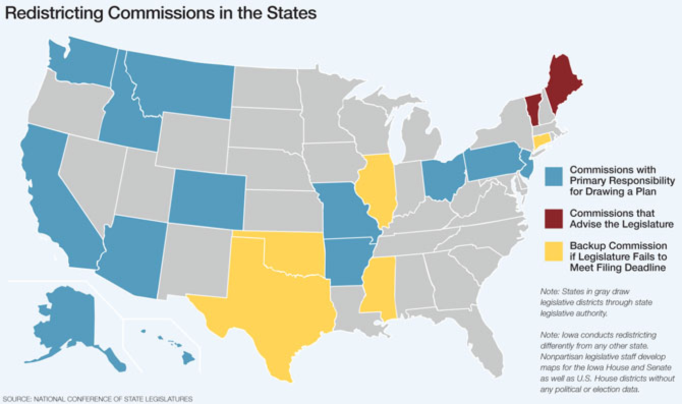
[3] Map describing the type of redistricting in each state
What is gerrymandering? Why should we care?
What is gerrymandering? Why should we care?
Gerrymandering is the practice of manipulating political boundaries to favor a certain group. This problem has been prevalent since the beginning of the country, when Patrick Henry attempted drawing the districts to oppose James Madison gaining a seat in Congress. The term was first created inspired by Massachusetts governor Elbridge Gerry, who signed a redistricting plan that obviously favored his party. Opposition thought that his district looked like a salamander which is where the word “gerrymandering” came from.
In[]:=
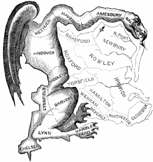
First Gerrymandering [1]
Gerrymandering is most typically done in two methods- cracking and packing. The meaning of these are just what they sound like. Cracking is when one party’s votes are split between districts to ensure they are not the majority. Packing is when one party’s votes are all concentrated in one district, to make it easier to win other districts.
There are many reasons that gerrymandering occurs.
There are many reasons that gerrymandering occurs.
◼
Cherry-picking voters
◼
Eliminating incumbents
◼
Eliminating challengers
◼
Skewing statewide representation
◼
Diluting minority voters
◼
Splitting communities
In[]:=
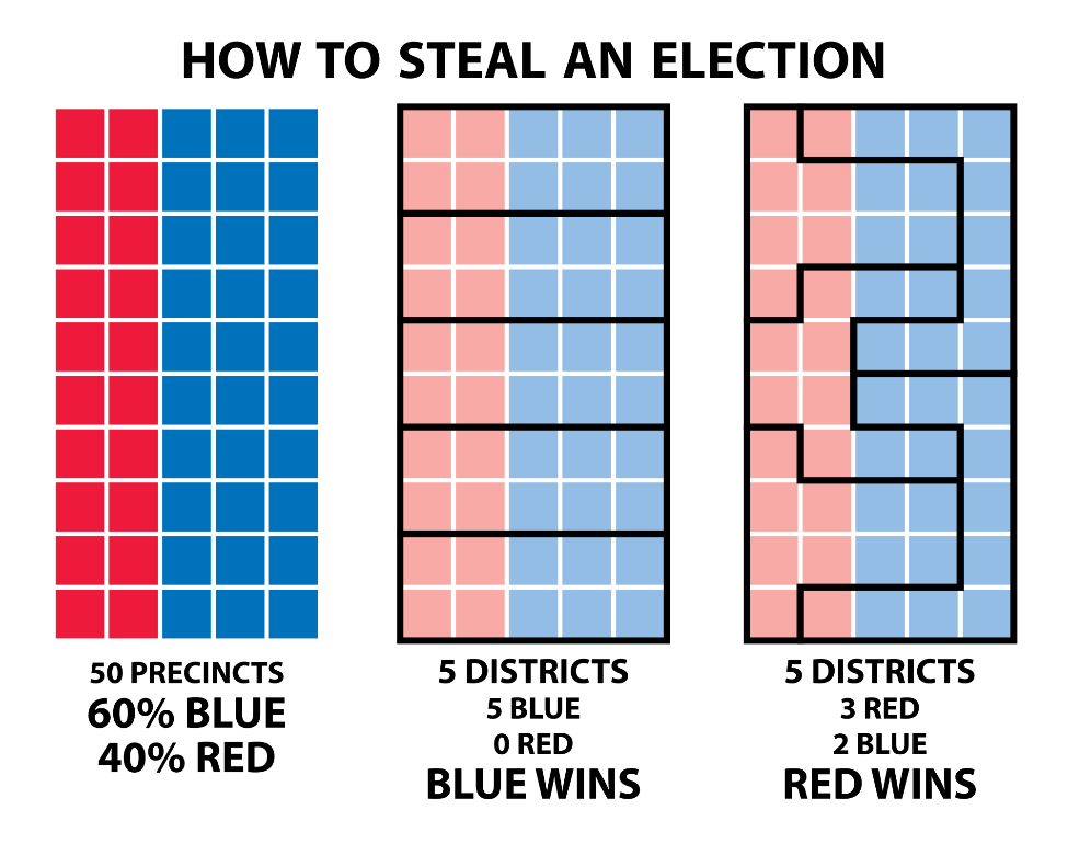
What gerrymandering looks like [2]
Combating Gerrymandering
Combating Gerrymandering
Judicial
Judicial
The role of the federal government in gerrymandering cases has been debated for years. In Davis v. Bandemer (1986), the Supreme Court held that gerrymandering could be held unconstitutional if the electoral system “is arranged in a manner that will consistently degrade a voter’s or a group of voters’ influence in the political process as a whole.” It did not hold that the court would take direct action against it.
In Vieth v. Jubelirer (2004), the court decided once again to reject the challenge due to lack of standards, but Justice Anthony Kennedy pointed towards the future that standards had the potential to emerge especially with computer-assisted districting. One such standard was proposed in Gill v. Whitford (2018), using the efficiency gap, which measures the number of wasted votes in an election. They argued that an efficiency gap of more that 7% was legally significant, but the Court still decided the evidence was insufficient. Most recently in Rucho v. Common Cause, the Court declared that “partisan gerrymandering claims present political questions beyond the reach of the federal courts.”
In Vieth v. Jubelirer (2004), the court decided once again to reject the challenge due to lack of standards, but Justice Anthony Kennedy pointed towards the future that standards had the potential to emerge especially with computer-assisted districting. One such standard was proposed in Gill v. Whitford (2018), using the efficiency gap, which measures the number of wasted votes in an election. They argued that an efficiency gap of more that 7% was legally significant, but the Court still decided the evidence was insufficient. Most recently in Rucho v. Common Cause, the Court declared that “partisan gerrymandering claims present political questions beyond the reach of the federal courts.”
State reform
State reform
As mentioned before states have been moving away from redistricting done solely by the state legislatures. Several states, such as Alaska, Arizona and California, employ nonpartisan independent commissions. The problem with this is that it is difficult to assume that the procedure for selecting members of the commission will truly be nonpartisan and resistant from political manipulation.
Non-governmental organizations
Non-governmental organizations
Fair Vote is a nonpartisan group that pushes or electoral reform across the United States. One of their main issues is gerrymandering, and the group supports legislative efforts that will reform the way we run elections and draw our boundaries. One of their proposed solutions is the Fair Representation Act where instead of having many districts with 1 representative, we have fewer districts with multiple representatives.
Many organizations have also emerged in the states themselves. For instance, in Virginia, One Virginia 2021 is working towards amending the State Constitution to take the power of redistricting from the state legislature to a Virginia Redistricting Commission.
Many organizations have also emerged in the states themselves. For instance, in Virginia, One Virginia 2021 is working towards amending the State Constitution to take the power of redistricting from the state legislature to a Virginia Redistricting Commission.
What has been done before on this subject in the math and computer science field?
What has been done before on this subject in the math and computer science field?
Duke Quantifying Gerrymandering
Duke Quantifying Gerrymandering
Duke Math has a nonpartisan research group that uses the ensemble method for outlier analysis. They generate a sample of nonpartisan maps and create questions of interest to assess these maps. They have been part of two gerrymandering legal cases in North Carolina and Wisconsin, as part of the argument against gerrymandering. They use the Markov chain Monte Carlo method to generate thousands of political maps creating distributions for analysis.
Princeton Gerrymandering Project
Princeton Gerrymandering Project
This nonpartisan group aims to use analysis to “understand and eliminate partisan gerrymandering at a state-by-state level”. They do so by writing up reports that use statistical and legal analyses that help groups strategize reform at a state level. Through improved communication, they believe that math and statistics can be used to back reform and legal cases. They have also gathered and cleaned data from thousands of counties to be put in a central repository called OpenPrecincts, to encourage the public to take action.
Purpose and Goals
Purpose and Goals
Our purpose
Our purpose
Our purpose is to combat gerrymandering and encourage fair democratic procedures to be used in all states. We want to display how statistical analysis can be used in reform efforts and legal cases as a tool to detect gerrymandering
Our goal
Our goal
We want to create an algorithm that can redistrict and account for equal population, compactness and continuity. We would also like to perform data analysis and calculations to quantitatively measure gerrymandering for simple comparison.
Creating a Map
Creating a Map
Random Graph
Random Graph
To represent a map, we decided to use the Graph function, which can show both distance and relationships between locations. Each node in the graph would represent a community or county that would then be put in a district for an election. In our project, we assume that there is an equal population for each community for simplicity. We first generate a RandomGraph.
Format Graph
Format Graph
To format the graph, we will randomly generate a number of votes for the “red” party and the “blue” party out of 100. The color of the vertex will depend on which party wins. The 100 can represent 100 people or a percentage of voters.
In[]:=
generatemap[a_, b_] := With[{graph = RandomGraph[{a, b}, EdgeStyle -> Dashed, EdgeStyle -> Gray, GraphHighlightStyle -> Automatic]}, (*create a random graph*) graph2 = Fold[ SetProperty[{#1, #2}, "Votes" -> <|"Red" -> #, "Blue" -> 100 - #, "Winner" -> If[# > 100 - #, "Red", "Blue"] |> &@ RandomInteger[{1, 100}] ] &, graph, Range[1, Length[VertexList[graph]]] ];(*Set random votes and winner of each vertex*) graph3 = Fold[ SetProperty[ {#1, #2}, VertexStyle -> If[PropertyValue[{#1, #2}, "Votes"][["Winner"]] == "Red", Red, Blue] ] &, graph2, Range[1, Length[VertexList[graph2]]]] (*Color the vertices according to the winning party*) ]
Redistricting and Calculations Function
Redistricting and Calculations Function
Our Algorithm
Our Algorithm
We created a districting algorithm that takes these nodes in the graph and randomly puts them into 3 equal continuous districts. Each district is denoted by a number 1-3 and the nodes are connected by a colored line. We perform various calculations after generating the districts.
Figure: Inputs, outputs and eventual results from the districting functions
We will use this complete graph, a graph where every pair of vertices is connected by an edge, in order to ensure that no error occurs in the reevaluations of this function. We recognize that this is unrealistic. In our algorithm, there is a flaw, where it will stop midway and return errors because it is not possible to create a continuous district when the remaining vertices have no adjacent vertices available to add to a district. We will account for these errors later when we generate our data.
Because every vertex is connected to every other vertex and we want to create districts that have the most efficient, the shape would be a circle divided into equal parts. Theoretically, the map this graph would represent would look something like what is shown below. Every section of the graph is connected to every other section at the center where they all meet.
Random Redistricting Algorithm
Random Redistricting Algorithm
District 1
District 1
Our algorithm creates one district, one vertex at a time .
This is what it would look like with the district 1 vertices labeled.
District 2
District 2
This same process is repeated to create the next district. The map and the remaining vertices are passed on the the districting algorithm for district 2. Otherwise the algorithm proceeds in the exact same way.
This is the map with 2 districts created:
District 3
District 3
The reason we chose not to just label the remaining points as district 3 is to ensure that the districts will be continuous. If it is not possible to be continuous, then the algorithm will have error that will be detected by our algorithm when we are generating data. We repeat the process again.
This is the map with all three districts labeled.
Now we have three important things-- a map with the vertices labeled with three districts (graph6), the list of vertices in each district (district1, district2, district3), and the vote counts for each party in each district (redvotes1, redvotes2, redvotes3, bluevotes1, bluevotes2, bluevotes3).
Count the votes and determine the winner
Count the votes and determine the winner
We now must determine which party won each district and determine the overall winner. We already have the counts of votes (redvotes1, redvotes2, redvotes3, bluevotes1, bluevotes2, bluevotes3), so we will use those to choose the winners. We use the color itself to denote a winner as a simpler visualization. In this step, we will also sum the votes for the map overall.
Determine the winners
Here, we can visualize the results of the countvotes[] function.
Format Map
Format Map
Now, we want to make our map more visually appealing, and incorporate the winning parties of each district. This function highlights the edges that connect vertices of the same district with the color that won that district.
Measuring Fairness: Efficiency Gap
Measuring Fairness: Efficiency Gap
Efficiency gap is a way to quantitatively measure gerrymandering, by comparing the number of wasted votes to total votes as a percentage. It was created by Eric McGhee and Nicholas Stephanopoulos. It has been theorized that if the efficiency gap is greater than 7 % then the map is likely to be gerrymandered.
There are two circumstances of a wasted vote:
There are two circumstances of a wasted vote:
◼
If the party won, the number of votes they did not need to win are considered to be wasted.
◼
If the party lost, then all the votes in that district for their party are considered to be wasted.
To demonstrate this calculation, we will use an example with 15 red voters and 15 blue voters that are split between 3 districts with 10 people. The following table shows the vote counts of each district.
Now, we can calculate the wasted vote totals for each party. If the party won, then any vote over the majority, which is 6, is wasted, so we subtract 6. If the party lost, then all of their votes are wasted. In the following chart, you can follow the process.
The efficiency gap is then calculated by the given by the absolute difference of the wasted votes of the two parties divided by the total amount of votes. This is the efficiency gap of this example.
This following function calculates the efficiency gap for the districts created by the districting functions.
Calculate efficiency gap
These are the results from carrying the function out:
Although efficiency gap can be a useful tool in measuring gerrymandering, it is not able to detect if these wasted votes are caused by gerrymandering or natural causes. For example, Democrats tend to win major cities with a overwhelming majority, which means there are a lot of wasted votes, but they are still supposed to be redistricted together.
Calculating Compactness: Reock Score
Calculating Compactness: Reock Score
The Reock score was used to quantify the amount of compactness of the districts. A challenge with this was that the regions of our map were supposed to be represented by distinct vertices, with the lines between the vertices only used as an identification for the orientation of each region (vertex). This made the idea of the ratio between areas ambiguous. However, the graphing of the map was essentially done to visualize the shapes of the districts, and it didn’t make sense to disregard the visual aspects of the map, such as the length or area between the vertices. We therefore decided to take into account the area and length between the vertices to calculate the Reock score.
Consider a random graph, representing an entire district:
The area of the district would be then computed, through creating a polygon with all of the vertices in the district, and getting the area of the polygon. To create a polygon that encompasses the entire district, the vertices of the polygon must be the outer vertices of the district. However, a major problem with this was that there wasn’t a good way to identify the outer vertices. WIthout identifying the outer vertices, problems like this would happen:
The order in which the vertices were entered into the polygon affected the shape of the polygon with the inner points. Therefore, the best solution was to find a region union of all polygons created with every permutation possible by the vertices in the district, and create another polygon with that.
Notice how the polygon created with the region union of all permutations of vertex coordinates resemble the outer convex shape of the district.
Then the smallest circle the encompasses the district was obtained by generating a list of every possible pairs of coordinates of the district, then getting the length of the distance between two coordinates furthest apart, which would be the diameter of the circle.
This was then combined into one function:
Then the smallest circle the encompasses the district was obtained by generating a list of every possible pairs of coordinates of the district, then getting the length of the distance between two coordinates furthest apart, which would be the diameter of the circle.
This was then combined into one function:
Calculate the Reock Score for one district
Calculate the Reock Score for all 3 districts and the average
These are the results Reock scores from our current example:
Summary of our results
Summary of our results
The following function was created to call all of the functions that we wrote with a single input of a map, which simplifies the process a lot:
Complete redistricting and calculations with a single input of a map
Now, this is all the code needed to complete the districting algorithm and following calculations.
We can also generate a summary of all the values and calculations we have completed.
This is a summary of the last time we called the redistrict[] function.
Generating Data
Generating Data
As mentioned in the introduction, Markov Chain Monte Carlos (MCMC) simulations have been used previously to generate thousands of iterations of redistricting plans. For instance, the group at Duke generated 19,184 redistricting plans for Wisconsin. Since we did not use MCMC and our computers are not powerful enough to generate such large amounts of data, we will use a simpler approach.
The next goal is to produce a valid data set of many iterations of our districting algorithm to perform analysis on. A flaw in our algorithm, as you may have found, is that it is not always able to produce a valid result with an incomplete graph. We will use a random graph in the next example.
The next goal is to produce a valid data set of many iterations of our districting algorithm to perform analysis on. A flaw in our algorithm, as you may have found, is that it is not always able to produce a valid result with an incomplete graph. We will use a random graph in the next example.
With a random graph like the one above, we will get a lot of invalid results from the districting algorithm failing. We will delete those cases that failed and delete the duplicate cases as well.
Repeat the redistrict[] function and check for duplicates and failure
We run the repeat algorithm and create the dataset. Oftentimes, we will get few results from running the algorithm many times. It is optimal to run with 9 vertices with many borders. We can see the size of the set with the Length function.
The data that is retrieved looks something like this. Here we give the first 10 graphs generated:
Now, we can generate lots of different redistricting plans to use for analysis and choosing the optimal plan. Since these are randomly generated results, they are going to vary each time the function is run. The more times the function is repeated, the more outputs you will get. We did not account for the identical maps where the district numbering is just switched.
The output of the data can be used to find the theoretical “best” plan--one with a low efficiency gap and a high Reock ratio.
If there were no districts and a simple vote was counted, this would be the result.
The output of the data can be used to find the theoretical “best” plan--one with a low efficiency gap and a high Reock ratio.
If there were no districts and a simple vote was counted, this would be the result.
Sometimes, the simple vote count results are different from the results from the redistricted map. This shows how drawing boundaries can really affect the political process.
Data Analysis
Data Analysis
The data generated can be analyzed through histograms. Our dataset is of course miniscule compared to that of professional researchers. In the previously mentioned analysis of Wisconsin’s redistricting plan the following histograms were generated using the number of elected Republicans. A map that is close to the center of the bell curve is less likely to be gerrymandered, because it is much more likely that the number of seats that were won by Republicans is representative of the people.
Distribution of election outcomes in the ensemble of Wisconsin redistricting plans using different election data-- Duke Quantifying Gerrymandering [4]
Reock Score
Reock Score
With our small dataset, it is difficult to generate a perfect bell-curve shape from a distribution. The closest and most useful measure is the Reock score average value. The following histogram and box and whisker plot show the distribution.
A larger value of Reock score indicates that the districts are more compact, since a score of 1 represents a perfectly compact district.
Efficiency Gap
Efficiency Gap
Efficiency gap is not a reliable measure of gerrymandering in our simulation due to the small scale. The value of efficiency gap will remain constant for those maps that have the same number of seats won by each party. For instance, for all the maps that have a 2-1 red district to blue district ratio, they will have the same value for efficiency gap. The resulting histogram from the dataset:
A larger efficiency gap indicates more wasted votes were present, and one party was additionally disadvantaged due to the boundaries.
Red Seats Won
Red Seats Won
With the same problem as efficiency gap, it is difficult to produce many different values for the number of red seats won, since the only possible values are 1, 2 , 3, so this is also not a particularly useful tool to detect gerrymandering.
We have been able to replicate a similar simplified version of an ensemble method of gerrymandering analysis. Due to the small-scale of our maps and data generation, we are unable to do in-depth analysis of our results.
Example
Example
To show the application of our project in the real world, we will use a theoretical example of a map called WolframLand. We assume that each colored area is a political subdivision that has 100 people. The map is numbered so that it is directly translated into the vertex index in our Graph.
WolframLand (Population 900)
WolframLand (Population 900)
Here we can see the votes for each party for each subdivision.
Now, we translate the visual map into a Graph, where each subdivision represents a vertex. We connect all the subdivisions that border each other with an edge. As you can see, our Graph loosely resembles the picture of the map.
This sets the vote numbers and colors the vertices according to the party that won the district.
With our input map, we can use our repeat[] function to generate randomly redistricted maps for WolframLand.
These are our results.
Let’s look at one specific example of a redistricted map.
This graph has been divided into districts such that Blue wins the election even though Red has more individual votes. This is an example of possible gerrymandering to favor the Blue party. It is also noticeable that there is a relatively high value of efficiency gap and a low value Reock score, which is characteristic of partisan gerrymandering.
We can also look at a map that would be considered to be more fair.
We can also look at a map that would be considered to be more fair.
Final Thoughts and Further Improvements
Final Thoughts and Further Improvements
Accomplishments
Accomplishments
Implications
Implications
Solved and Ongoing Challenges
Solved and Ongoing Challenges
Future Work
Future Work
Overall, future work involves making the algorithm more efficient and realistic.
◼
Allow the function to take in an input for number of districts, so we can redistrict maps into 4, 5, or any number of districts.
◼
Modify the function to allow for each vertex to have a different population size, which is more representative of actual counties and political subdivisions.
◼
Scale the map sizes up and eventually take in an input of a real political map of a state.
◼
Take out the data where the districts are the same and merely the order of district numbers is changed.
◼
Implement a Markov Chain Monte Carlo method for redistricting to have more complete and accurate data.
Sources
Sources