A metafluid with multistable density and internal energy states
by Ofek Peretz, Ezra Ben Abu, Anna Zigelman, Sefi Givli and Amir D. Gat.
by Ofek Peretz, Ezra Ben Abu, Anna Zigelman, Sefi Givli and Amir D. Gat.
Article abstract
Article abstract
Investigating and tailoring the thermodynamic properties of different fluids is crucial to many fields. For example, the efficiency, operation range, and environmental safety of applications in energy and refrigeration cycles are highly affected by the properties of the respective available fluids. Here, we suggest combining gas, liquid and multistable elastic capsules to create an artificial fluid with a multitude of stable states. We study, theoretically and experimentally, the suspension’s internal energy, equilibrium pressure-density relations, and their stability for both adiabatic and isothermal processes. We show that the elastic multistability of the capsules endows the fluid with multistable thermodynamic properties, including the ability of capturing and storing energy at standard atmospheric conditions, not found in naturally available fluids.
Introduction / Overview
Introduction / Overview
The purpose of this notebook is to obtain an analytical understanding of the thermodynamic behavior of a multistable structure composed of a series of bistable elements coupled with encapsulated gas. In section 1 we derive the pressure-volume relation for a single capsule and its internal energy at equilibrium as a function of the external pressure. In section 2 we simulate the Bryton refrigeration cycle using the proposed metafluid as a refrigerant in comparison to a standard, gas-only, refrigerant currently in use.
Nomenclature
Nomenclature
This code presents analytic solution for the case of metafluid consists of multistable capsules and was used to generate the data for the simulation presented in Fig. 2-4 in the paper.Nomenclature:n -The number of bistable elements in each capsule.Φ - number of capsules per-unit-mass.vs1 -The volume of the element at snap-open pressure.vs2 - The volume of the element at snap-close pressure.k1 - Stiffness at phase 1.k2 - Stiffness at phase 2.psopen -Snap-open pressure value.psclose -Snap-close pressure value.pa -Atmospheric pressure.γ - Adiabatic indexper={n1,ns,n2} - Number of elements in phase 1, spinodal and phase 2 respectively.Vs - The total volume of a single capsule. - The elastic energy per unit mass. - The gas energy per unit mass.
U
el
U
gas
Constants
Constants
In[]:=
n=18;γ=7/5;Φ=16;pa=1;vs1=4/10;vs2=8/10;k1=10;k2=10;psup=25/100;psdown=-25/100;v0=6;(*(n/2)(vs1+vs2);*)
Section 1 - Equilibrium and internal energy calculations
Section 1 - Equilibrium and internal energy calculations
Pressure-volume relation for a single capsule is derived for a tri-linear bistable elements (composed of three regions - 1,s,2) coupled with the behaviour of the encapsulated gas.
In[]:=
per=Reverse[Pick[Tuples[Range[0,n],3],Tuples[Range[0,n],3].{1,1,1},n]];per=Pick[per,Thread[per〚;;,2〛<2]];Nper=Length[per];perStable=Pick[per,Thread[per〚;;,2〛0]];perUStable=Pick[per,Thread[per〚;;,2〛>0]];perStableIndex=Table[If[per〚i,2〛0,i,Nothing],{i,1,Nper}];perUNStableIndex=Table[If[per〚i,2〛≥ 1,i,Nothing],{i,1,Nper}];ks=;pI[v_]:=k1(v-vs1)+psup;ps[v_]:=ks(v-vs1)+psup;pII[v_]:=k2(v-vs2)+psdown;Peli[i_,v_]:=-If[i1,pI[v],If[iNper,pII[v],ps[v]]];v1vs=vv1/.First[Solve[ps[v]pI[vv1],vv1]];v2vs=vv2/.First[Solve[ps[v]pII[vv2],vv2]];v1s[vv_]:=v1vs/.{vvv};v2s[vv_]:=v2vs/.{vvv};Vc[i_,v_]:=If[Or[i1,iNper],n v,per〚i〛.{v1s[v],v,v2s[v]}];Pgas[V_,V00_]:=pa;dPgas[V_,V00_]:=Derivative[1,0][Pgas][VV,V00]/.{VVV};Pitot[i_,vv_,V00_]:=Pgas[Vc[i,vv],V00]+Peli[i,vv];kbar[i_]:=;kgbar[l_,i_,v00_]:=-dPgas[Vc[i,l],v00]+;stability[i_,l_,v00_]:=If[per〚i,2〛0,1,If[per〚i,2〛>1,0,If[kbar[i]<0,If[kgbar[l,i,v00]>0,1,0],0]]];vrange=Join[{{0.001vs1,vs1}},Table[{vs1,vs2},{i,2,Nper-1}],{{vs2,2vs2+vs1}}];UItemp = Integrate[pI[x], {x, 0, v}];Ustemp = Integrate[ps[x], {x, 0, v}];UIItemp = Integrate[pII[x], {x, 0,v}];UI[vv_] := ((UItemp) /. {v -> vv}) - (UItemp /. {v -> vs1});Us[vv_] := (Ustemp /. {v -> vv}) - (Ustemp /. {v -> vs1}) + UI[vs1];UII[vv_] := (UIItemp /. {v vv}) - (UIItemp /. {v -> vs2}) + Us[vs2];Uel[i_,v_]:=per〚i〛.{UI[If[i1,v,v1s[v]]],Us[v],UII[If[iNper,v,v2s[v]]]};Ugass[vv_,V00_]:=Integrate[Pgas[vv1,V00],vv1]/.{vv1vv};Ugas0[V00_]:=Ugass[V00,V00]; Ugas[V_,V00_]:=Ugass[V,V00]-Ugas0[V00];Ufrange=Join[{{Pitot[1,vs1,v0],3}},Table[{Pitot[i,vs1,v0],Pitot[i,vs2,v0]},{i,2,Nper-1}],{{Pitot[Nper,vs2,v0],2}}];vVSp[i_,p_,V00_]:=Max[v/.NSolve[Pitot[i,v,V00]p&&0.99vrange〚i,1〛≤ v≤ 1.1vrange〚i,2〛,v]];Utot[i_,p_,V00_]:=Ugas[Vc[i,vVSp[i,p,V00]],V00]+Uel[i,vVSp[i,p,V00]]-pVc[i,vVSp[i,p,V00]]-(vs1+vs2);UgasVSp[i_,p_,V00_]:=Ugas[Vc[i,vVSp[i,p,V00]],V00]-pVc[i,vVSp[i,p,V00]]-(vs1+vs2);
psup-psdown
vs1-vs2
γ
V00
V
-1
peri.,,
1
k1
1
ks
1
k2
-1
peri.,,
1
k1
1
ks
1
k1
n
2
n
2
Results
Results
External pressure (p) Vs Equivalent density ρ
External pressure (p) Vs Equivalent density ρ
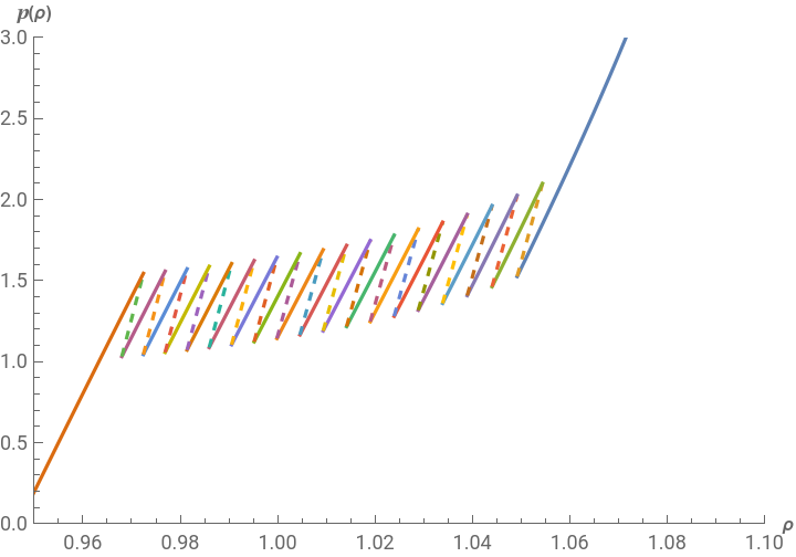
In the following figure, we show the pressure-density relation a metafluid with multistable capsules. Dashed lines represents unstable permutations, full line represents stable permutation.
In[]:=
plotrangePvsρ={{0.95,1.1},{0,3}};plotFvsL=ShowTableParametricPlot,Piecewise[{{Pitot[i,l,v0]+pa,stability[i,l,v0]1}},None],,Piecewise[{{Pitot[i,l,v0]+pa,stability[i,l,v0]0}},None],{l,vrange〚i,1〛,vrange〚i,2〛},PlotRangeplotrangePvsρ,PlotStyle{{ColorData[97,i]},{ColorData[97,i],Dashed}},AspectRatio23,AxesLabel{"ρ","p(ρ)"},{i,1,Nper}
3062
3072+2Φ(Vc[i,l]-2v0)
3062
3072+2Φ(Vc[i,l]-2v0)
Out[]=
Internal energy (U) Vs External pressure (p)
Internal energy (U) Vs External pressure (p)
The following figure shows the internal energy of the system as a function of the external pressure . Energy difference between different permutations at the same pressure values is observed, allowing the system to store and release energy at atmospheric conditions.
p
ex
In[]:=
plotrangeUvsP={{0.1,0.9},{2.5,4.5}};plotUvsF=Show[Show[Table[ParametricPlot[{p,Utot[i,p,v0]},{p,Ufrange〚i,1〛,Ufrange〚i,2〛},PlotRangeplotrangeUvsP,PlotStyleColorData[97,2],AxesLabel{"",""}],{i,perStableIndex}]],Show[Table[ParametricPlot[{p,Utot[i,p,v0]},{p,Ufrange〚i,1〛,Ufrange〚i,2〛},PlotRangeplotrangeUvsP,PlotStyle{ColorData[97,3],Thin}],{i,perUNStableIndex}]],AspectRatio2/3]
P
ex
U
tot
Section 2 - Refrigeration cycle
Section 2 - Refrigeration cycle
In this section, we simulate the Bryton refrigeration cycle using the proposed metafluid as a refrigerant in comparison to a standard, gas-only, refrigerant currently in use.
Results
Results
Refrigeration cycle
Refrigeration cycle
In the following figure, we show simulation of a Brayton refrigeration cycle (colored lines for metafluid and blue line for reference gas-only refrigerant).
Left panel shows pressure-volume relation and right panel shows Temperature - Entropy relation.
Coefficient of operation is calculated in both cases.
Left panel shows pressure-volume relation and right panel shows Temperature - Entropy relation.
Coefficient of operation is calculated in both cases.
Contact information
Contact information
Detailed analysis is provided in the main text as well as the supplamentary information
For more info, contact:
Ofek Peretz, ofekperetz@campus.technion.ac.il
For more info, contact:
Ofek Peretz, ofekperetz@campus.technion.ac.il