(a failed first experiment?)
(a failed first experiment?)
Introduction
Introduction
During a total solar eclipse, it is sometimes possible, when standing in a rare location, to observe two concurrent Baily's beads. Astronomy enthusiasts call this phenomena a “double diamond ring”, and attribute its occurrence to height deviations on the lunar limb.
Michael Zeiler and Ernie Wright have agreed on their calculations of the odd umbral shape, almost polygonal with pronounced corners. The original discoverers also claim these corners correspond to the rare locations for viewing double diamond rings. This is an exciting prediction that could be tested this year April 8, for example in Carbondale, IL.
However, it’s been a surprise to many of us that such predictions are even possible, and we’re hoping to gain more insight about the mathematics by obtaining a simplified proof of concept. Source code from Zeiler and Wright would probably be better, but who has time to check difficult and intricate necessities? That’s why we’re trying to boil things down to the bare essentials.
A simple eclipse model
A simple eclipse model
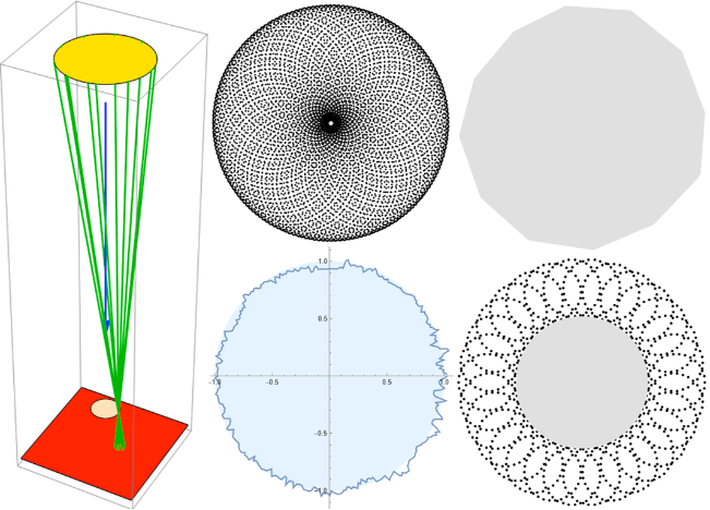
For a first idea, we can probably forget about the earth entirely, except that its centroid fixes an equatorial plane to the normal vector defined by the difference between the sun and moon. This is the so-called "fundamental plane", which has (possibly-non-intersecting) cross sections for the earth, the sun, and the moon. Just before the eclipse, a schematic view could look something like this:
Out[]=

This sketch is obviously not to scale, but shows the necessary dimensions: The normal vector in blue, and the fundamental plane in red. As the moon moves around the earth, the blue vector moves too, and eventually points to the earth.
The next assumption may be problematic, but let’s address that later. Rather than keeping a spherical sun and moon, we will reduce to “limbs only”, which means taking a cross section from each body’s equatorial plane.
The Sun’s cross section should be almost a perfect circle, not just because of its incredible size, but also because the surface of the sun is a plasma, which isn’t rigid enough to support permanent height variation. The moon, on its own, has its mountains, valleys, no rivers but yes to detectable water molecules. Here we give an example (from Stephen Wolfram and Jose), with 30x exaggeration what the lunar limb could technically look like:
Out[]=
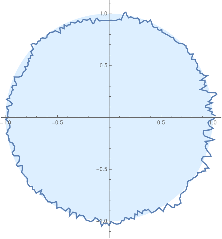
This is too much to start with. At first, we really need to perform a control experiment using circles only. This can be done quite easily on pencil and paper, but it can be easier to see with three-dimensional computer graphics. Our circle-circle-plane mathematical model can be defined in terms of only four parameters:
In[]:=
ra=1;rb=1/3;dap=10;dbp=1;
Out[]=

The four parameters are respectively: the ray-casting-circle radius, the occulting-circle radius, and the vertical height of both circles measured from the fundamental plane.
Again, parameters have been chosen for visibility sake, and changing them does not affect qualitative features of the model. The most important feature is that the smaller circle closer to the fundamental plane will occult rays cast from the larger, more distant circle. It is in some sense a projective geometry, but we always have uncountably many pencils to integrate over.
The outer product of a circumference with a conic section can indeed be chosen here in two distinct ways. Either one of the circles is taken as a cross section, while the other is tangent to the locus through which flows all tangents of a particular conic. The alternatives can be drawn out as follows:
Out[]=
 ,

In neither of these two alternatives is the section on the fundamental plane equivalent to the umbra itself, but in both cases the umbra can be calculated by integrating a function over the tangent circle. The umbra can be defined this way, but it is also just the shadow cast by the occulting body (a circular moon in this case).
In the first partial model, points interior to the circle on the fundamental plane can never see the casting point on the solar limb. Points outside the circle always can see the casting point. The total umbra is then obtained by taking the mutual intersection of all such partial umbras.
In the second model, points interior to the circle on the fundamental plane can always see at least one point on the solar limb. Outside the circle, we don’t know if it’s light or dark. To get the shadow spot we need an extra step. Take the union of known bright spots over the occulting limb, and divide this region out of the plane. If we get exterior and interior regions (i.e. containing
or not the point at infinity), then the interior region is the shadow spot.
or not the point at infinity), then the interior region is the shadow spot.
The second model is not as immediately intuitive from theory, but makes more sense when you see total projected data such as this discrete approximation:
Out[]=
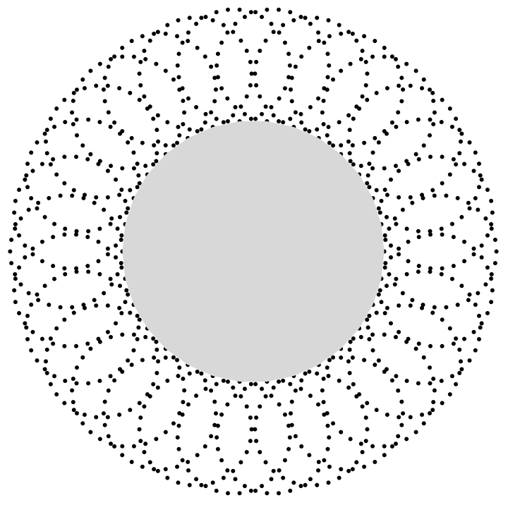
Here the black points are obtained by intersecting an outer variety of conic tangents with the fundamental plane. The umbra in light gray is obtained as the convex hull of all points after a 1/z Mobius transformation.
For a next experiment, we can put a notch in the circle by cutting out 5 degrees with a step function:
Out[]=

Now we repeat the same calculation to obtain the umbra, and it is indeed polygonal, but only because our algorithm using ConvexHullRegion malfunctions after Mobius inversion:
This is a nice illustration how easy it is for a clever idea to end up mistaken, and gives the skeptics among us some pause: What if Zeiler and Wright both made a mistake similar to this one? That seems unlikely, but what do we know if a proof isn’t made available?
Well, anyways, we can see what’s happening. When an occulting point is perturbed off the limb, it’s bright spot perturbs proportionally. Undoubtedly, there’s a law of similar triangles, which we’ve yet to write down, but could yield predictive rationals.
Let’s leave the theory for the interested reader to work out (and post below?). We can push the experiment forward a few steps by putting moon data into our math calculation, here shown with 30x exaggeration:
And here shown with more realistic parameters:
At this scale it’s difficult to see the umbra shape, so let’s try extracting it:
Here we’ve got a polygon result, but again, is this just because of our loose usage of complex planar transformations? We should be able to check by varying the discretization parameter, and would expect a smoother spot with higher resolution sampling. That is indeed what happens:
While the previous approximation was plausibly similar to Zeiler and Wright results, this lumpy circle is close enough to circular to doubt that our calculations have captured statistically significant corners where “double diamonds” could be found.
CITE THIS NOTEBOOK
CITE THIS NOTEBOOK
Eclipses and conic sections
by Brad Klee
Wolfram Community, STAFF PICKS, March 13, 2024
https://community.wolfram.com/groups/-/m/t/3139774
by Brad Klee
Wolfram Community, STAFF PICKS, March 13, 2024
https://community.wolfram.com/groups/-/m/t/3139774