Introduction
Introduction
The I Ching (易經) is an ancient Chinese divination manual, predating both Lao Tzu and Chuang Tzu. It contains = 64 oracle readings, which are meant to be consulted in the style of “choose your own adventure”. Perhaps it would be okay to read the I Ching reflexively, by picking and choosing hexagrams to follow important storylines or conditions in nature. More likely we’re better off planning for the future with randomized transitions from one hexagram to the next. However we decide to dive into the mystery, the introduction to David Hinton's translation says the following:
6
2
“To read the I Ching like this, as a mystery given evanescent shape in poetry and philosophy, is to return to the origin place where heaven and earth interact in that all-encompassing generative present, to our own primal origins, our place at the wellsprings of change. It is, in fact, to become dragon again.”
By accepting completely randomized transitions, we will end up in the field of probability and statistics, wondering what our acceptance function should look like.. Minimally speaking, all that we need is a probabilistic method for deciding between Yin (陰) and Yang (陽), which can be repeated six times to obtain a hexagram consisting of a stack of lines, either unified (陽) or divided (陰). The weight of history is also in play, so the obvious minimal model of six coin flips can not work as even the simulacra of an authentic practice. Indeed, the situation is not as simple as it first appears. Not only are there more than binary outcomes to consider, the way to get to those outcomes is not an optimized path, but rather, a road less traveled.
Fortunately for us, David’s translation has an entire section on “How to consult the I Ching”, which gives two methods: by “shaman-flower” (筮) or by coin (These two methods are also found on wikibooks, if you’d prefer). Both methods require hexagrams lines in quarter phases, not only as full or empty (少陽 or 少陰), but also alternatively as waxing or waning (老陰 or 老陽). A two-flip coin model would get us equal probabilities for 少陽, 少陰, 老陰 and 老陽, but again, this won’t lead to traditional results. A three coin method makes probabilities P(老陰)=P(老陽) more unlikely than P(少陰)=P(少陽). This is a bit better than two coins, but still relatively tame compared to the shaman flower method, which typically has probabilities P(少陰)>P(少陽)>P(老陽)>P(老陰).
In this memo we consider the shaman-flower method as a combinatorial solitaire, and analyze how different choice functions affect outcome probabilities. Once we have an acceptable probabilistic model, we will use it to simulate the casting of hexagrams and their completion phases.
The “Shaman-Flower” Method
The “Shaman-Flower” Method
The Shaman-Flower solitaire starts with a heap (蘊) of 50 dried yarrow stalks. If you don’t have any yarrow stalks, that shouldn’t be too much of a problem during June and July at least. Just go outside and find them growing by the side of the highway somewhere, collect them, trim the flowers and leaves, dry them and cut them to similar size. If it’s not June or July, perhaps Etsy will be a better bet (they should have seeds). In any case, actually obtaining fifty yarrow stalks is not necessary for a simulation of the experiment.
Our simulation starts with an initialize function, 初始化筮, which sets up an association with six keys: the yarrow heap (蓍蘊), the graveyard (太極), the left hand (左手), the right hand (右手), the score (比分) and the result (结果). Initially, everything is empty other than the yarrow heap:
In[]:=
初始化筮[]:=Association"蓍蘊"->50,"太極"->0,"左手"->0,"右手"->0,"比分"->{},"结果"->"無"
To continue the solitaire, we need an iterator 迭代筮, which identifies a present state (状态) and then lists all possible next states. In practice, this is done using a Which statement that tests properties of the input 状态, and then transforms them accordingly.
For example, the first move is always the same:
In[]:=
迭代筮状态_:>Module{各下状态},Which状态["太極"]==0,各下状态=状态;各下状态["蓍蘊"]--;各下状态["太極"]++;{各下状态}(*morerulesneeded...*);
One of the yarrow stalks goes from the heap to the graveyard. Due to ordering of Which, the next move only triggers if the first does not:
In[]:=
迭代筮状态_:>Module{各下状态},Which(*previousrulehere,*)SameQ0,状态["左手"],状态["右手"],各下状态=状态;各下状态["蓍蘊"]=0;If各下状态["太極"]==1,各下状态["太極"]++;MapReplacePart各下状态,"左手"->状态["蓍蘊"]-#,"右手"->#-1&,Range2,状态["蓍蘊"]-1;
Here we require that the right pile still has finitely many items after subtracting one. When the graveyard has only one item, we move the extra stalk directly there, thus leaving 48 items in either the left or right hand. Once the fates are split, they need to be scored and recombined, using essentially a modulus function:
In[]:=
迭代筮状态_:>Module{各下状态},Which(*previousruleshere,*)SameQ0,状态["蓍蘊"],各下状态=状态;IfOrMod各下状态["左手"],4==0,AndMod各下状态["左手"],4==3,Length[各下状态["比分"]]>0,AppendTo各下状态["比分"],2;各下状态["蓍蘊"]=-8;各下状态["太極"]+=8;,AppendTo各下状态["比分"],3;各下状态["蓍蘊"]=-4;各下状态["太極"]+=4;;各下状态["蓍蘊"]=Plus各下状态["左手"],各下状态["右手"],各下状态["蓍蘊"],BooleLength[各下状态["比分"]]>1;各下状态["左手"]=各下状态["右手"]=0;IfLength[各下状态["比分"]]==3,各下状态["结果"]=$分到爻[Total[各下状态["比分"]]];;{各下状态};
This branch of the Which statement treats the first reduction round differently than the next two. When three partial scores (比分) are accumulated, then the same code sets the result (结果) according to the following dictionary for converting from total score:
In[]:=
$分到爻=Association6->"老陰",7->"少陽",8->"少陰",9->"老陽";
Finally, the iterator is complete by specifying the termination conditions at highest priority, which allows them to supersede any more rounds of branching and merging:
In[]:=
迭代筮状态_:>Module{各下状态},WhichLength[状态]==1,{},UnsameQ状态["结果"],"無",{Association["结果"->状态["结果"]]}(*,previousruleshere*);
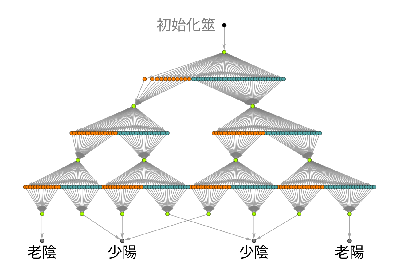
Once the iterator is fully defined, we can compute the graph seen above and the stratification of its vertices:
In[]:=
Withg1=ResourceFunction["FixedPointGraph"]迭代筮,初始化筮[],strat=ResourceFunction["VertexStratify"][g1];Length/@strat
Out[]=
{1,1,47,2,80,4,136,8,4}
Indeed it’s easy to see the levels riffle between expansive and contractive. Expansive levels have the following vertex counts:
In[]:=
Length/@strat[[{3,5,7}]]
Out[]=
{47,80,136}
Which are explained by binomial branching of yarrow stalks going into the left and right hands:
In[]:=
{{Length[Range[2,48]]},{Length[Range[2,44-1]],Length[Range[2,40-1]]},{Length[Range[2,40-1]],Length[Range[2,36-1]],Length[Range[2,36-1]],Length[Range[2,32-1]]}}Total/@%
After merging, state counts per level go back to powers of two associated with the binary variable that goes into the score column:
From a coarse-grained perspective, most of what we need from the full game graph is contained in the binary-branching subgraph over the green nodes:
According to modulus properties of the iterator in its branch and merge steps, we can naively estimate the probabilities on each edge of this graph:
Using our favorite game-solving tool, WFR`DirectedAcyclicEvaluate, we can then convert edge probabilities into probabilities on each vertex:
With no mergers and so few vertices, this subgraph makes an easy example. We can check by inspection that DirectedAcyclicEvaluate is computing partial probabilities correctly:
Each vertex probabiity equals the product of it’s input edge probability with it’s parent node probability. All edge probabilities, grouped by initial vertex, sum to one; thus, the sum of probabilities over each vertex level also equals one:
We mainly care about results on the final level, which need to be accumulated by result:
Compare with the probabilities obtained by flipping three coins:
The percent differences are already considerably large, indicating that significantly different results will be obtained using coins or dried yarrow stalks:
Just by observing denominator = 16 in the naive shaman-flower probability estimates, it seems that at least four coin flips would be needed to determine one hexagram line to similar precision. However, the naive estimate makes assumptions about approximating expansive probabilities. Is the naive estimate realistic? How can we prove that it is?
Binomial heap division
Binomial heap division
A true solitaire involves a selfish one player who continually makes choices when given alternatives. Considering that it’s always impossible for a person to act as a selfless probabilistic machine, the shaman-flower method can be seen as a solitaire. Yet the purpose of the game is to enter into a totally integrated cosmos where player and game are completely indistinguishable. Other than meditative absorption, how could this possibly happen? Let’s just do the math and find out.
Clearly if a vertex has only one out component, it must be followed. If there are multiple out components from one vertex, then we need a distribution of partial probabilities summing to one . An unrealistic but simple choice is the uniform distribution :
Again, we can feed the edge weights into DirectedAcyclicEvaluate, which then computes the corresponding probabilities on each vertex:
For the most part, we just care about the results:
Again they are significantly different from the naive estimate:
To ascertain the reason, let’s look more closely at the binary tree obtained from the subgraph of lime green vertices only:
Quite obviously, the edge probabilities are not multiples of 1/4. This happens because of edge effects related to our assumption that neither right nor left hand can ever go empty. For example, on the first and second levels we have:
By modifying the allowable Range inputs, we can force agreement with naive estimates:
However, if we accept empty-hands moves, then we need new rules explaining that an empty hand should always result in the lesser score of 2. If at all possible, we don’t want to second guess tradition by adding new rules. Fortunately for us, edge effects are not serious when choosing better edge weights for fairly dividing yarrow heaps roughly in halves.
A very sensible choice is to use a binomial distribution, which essentially assumes that every yarrow stalk has an equal chance of going into either the left or right hand:
At the first expansive stage, we can already see that a hand with 10 or fewer stalks is extremely improbable:
By the numbers, we’re over 15,000 times more likely to end up at least ten stalks in both hands:
And on subsequent iterations, similar conditions continue to hold:
In this probabilistic model, whether we allow or disallow hands with zero yarrow stalks really does not matter, because in practice, the probability of obtaining an empty hand is bounded above by about one part in a billion:
Let’s now accept this model as is and move on to calculating coarse grained weights:
We’ve calculated some monstrous fractions, which don’t fit neatly on the graph. If we ask for only a few digits of the fractional expansion, then it looks like we’ve closely recovered the naive result:
In this case, the percent differences are 10 or 100 parts per million:
In one person’s lifetime, it probably makes absolutely no difference whatsoever if four coins are flipped or if the shaman flower method is performed as close to randomized binomial choosing as possible. If a coin and yarrow stalks are available, the most reliable heap-splitting procedure would involve flipping the coin to decide, for every yarrow stalk, whether it would belong in the left or right pile.
Practice considerations aside, we have everything we need to move forward with a simulations of the flower-shaman method. Simulations can skip intermediary steps, so results can be obtained with much more rapidity. This is obviously not a good idea for serious meditative practice, but we can do more of that later once we understand how the math works inside of a computer.
Divinulation
Divinulation
Now that bots like ChatGPT are capable of reading the I-Ching among a vast library of world classics, we can expect a big future for the field of “Divinulation” (divination simulation). For now, the LLM’s are not trustworthy about probability and statistics, so we can’t expect them to give statistically-unbiased readings. Fortunately for us, such results are easy to obtain with only a few lines of Mathematica code. For example, here’s a random hexagon obtained using our special binomial statistics:
And indeed we get the same result using naive statistics as well:
Reading the words left-to-right and stacking lines bottom-to-top, we obtain an image and it’s transformational partner:
Consulting with David’s translation, we can guess that Woman’s Generative Power will go toward exhaustion in the future. Impressively, this reading seems not only immediately relevant to the news cycle, but also a foregone conclusion of the human body typically ending up weak and depleted by the end of its lifetime.
Before we get in too much trouble with sexist dragon talk, let’s get back to the facts. We can test how long it will take for the two approximately equal probabilistic models to give a different result for just one line:
If we assume that six lines are computed once per month, then we could estimate about ten lifetimes before a discrepancy would ever be likely to arise:
Most people probably wouldn’t go through even two or three reincarnations as such a serious I Ching practitioner, so again, it seems absolutely fine to use naive statistics for casting hexagrams:
For a final experiment, we can try the reflexive approach. For example, recently I’ve had a success breeding Hercules beetles, raised the larvae through pupation, and released at least one of them back to nature. After a few years of hard work, my personal ecological bias takes me to the ninth hexagram “Delicate Nurturing”. We can cast repeatedly until obtaining this hexagram:
After about 60 or 70 tries, we obtain the expected pre-image, and a mostly unpredictable transformation to the eleventh hexagram “Devotion”:
Truly wonderful discovery! Devotion is one of two perfectly balanced hexagrams, and it’s much easier to deal with as a potential future than would be its parity opposite “Obstruction” (#12). If you make Devotion, “天人合一”, so expect free and easy wandering. If you encounter Obstruction instead, after many changes 土 must eventually triumph over 天, but in the short term, 人 can not triumph over either.
Again, let’s not get too distracted by dragon talk. There is still at least one interesting question to answer. Say that we have hexagram 9. What are the relative probabilities of obtaining either hexagram 11 or 12 as a result of casting with quarter phases? Of course, the answer depends on the choice model. First we reverse and re-normalize stats:
Then we can compute the probability of a transition, and it’s mirror image:
Then we find that if you start from “Delicate Nurturing”, you’re about 10x as likely to end up at “Devotion” as you would be to end at “Obstruction”:
If that doesn’t make natural sense to you, perhaps the I Ching is just not your cup of tea. In that case, let’s not end with dragon insight, but rather with a more complete calculation, the entire transition matrix:
It’s rows sum to one:
It’s columns are not normalized, indicating that some destinations are more popular than others:
Indeed this is unavoidable due to the relatively higher cost of transforming 老陰 into 少陽. As a check on values, we can make sure to have recovered our previous result:
And as a next step in statistical exploration, we find the most and least likely transformations:
The most likely is ䷁→䷁ and the least likely is ䷁→䷀. Of course, on closer observation, the most likely transformation of any character is into itself:
And generally, the next most likely transformation will have only one line changed, a 陽 into a 陰 where possible. Thus the least likely transform is the one that changes six 陰 into six 陽. Finally, let’s take a look at the multiplier between most and least probable items per row:
Hmm, curiously similar structure to the earlier plot... Some hexagrams are much easier to transform out of then others would be. What’s the reason for this trend?
In general, the more 陰 lines a hexagram has, the more difficult it will be to change. The reason is that a change 少陰→老陰 decreases the probability by a factor of 7, while a change 少陽→老陽 only decreases probability by a factor of 5/3. Taking our earlier example, we either change two yang lines or three yang lines plus one yin line. This gives us another way to computer the likelihood ratio:
In our previous case of the ninth hexagram, it’s now become easier to understand why five alternatives are most likely, and why ten alternatives (including ䷊) are second most likely. As 25/9 is still less than seven, 5 and 10 are just subsequent binomial coefficients. We can tabulate transformational outcomes in order of decreasing likelihood:
Then we see that the binomial pattern continues to the fourth row, until 7< 625/81 in the fifth row, at which point “Heaven” can be obtained relatively easily. It’s quite a temptation to spend more time investigating the transition matrix for clues of what could happen next, but we’ve simply run out of time today.
In conclusion, we’ve shown how much fun we can have and how much we can learn from Computational divination or “divinulation”. Our analysis via binomial choosing proves the validity of four naive partial probabilities regardless of edge effects that should usually not occur in practice. We have also shown how to use the partial probabilities to obtain quarter-phased hexagram lines, and to predict pairs of relevant hexagrams by repeating one function call six consecutive times. For example, here’s another pair:
Fall will change into winter, but for now it’s only late July. A logical next step would be going out into the world in search of more yarrow stalks. There’s still enough time for collecting and drying. Perhaps by November, more authentic experiments with the I Ching will be possible. Wouldn’t it be great if all of life’s important decisions could be seen as no more consequential than a series of clumsy accidents caused by our inability to divide yarrow heaps into exactly equal portions?
code
code
CITE THIS NOTEBOOK
CITE THIS NOTEBOOK
Multiway Analysis of "Shaman-Flower" Method
by Brad Klee
Wolfram Community, STAFF PICKS, July 29, 2024
https://community.wolfram.com/groups/-/m/t/3237184
by Brad Klee
Wolfram Community, STAFF PICKS, July 29, 2024
https://community.wolfram.com/groups/-/m/t/3237184