Analyzing unemployment in India during COVID-19 pandemic
by Ashika Deb
Miranda House, University of Delhi, India
by Ashika Deb
Miranda House, University of Delhi, India
Unemployment gives birth to several social and economic problems and the COVID-19 pandemic has exposed and exacerbated existing inequities in the labour market heightening this issue. The pandemic has changed the course of the world and due to drastic economic changes, the state of employment has inevitably changed globally, more so in developing countries. Power and privilege are major determinants of who is at risk for precarious work, with historically marginalized communities being disproportionately vulnerable to these job conditions. The pandemic worsened the situation for millions who were already dangling between the line of poverty and helplessness leading to massive job losses and a huge talent vacuum. The problem of millions of helpless migrant labourers losing their homes due to lockdown and loss of jobs has also plagued India.
This project will focus on studying unemployment data in India and try to examine relations between the various factors that may have affected the unemployment during the pandemic. Towards this end, we will examine available data from official sources and utilize Wolfram Language capabilities to perform an exploration analysis and draw out meaningful statistics from them. Furthermore, we would like to perform sentiment analysis on twitter data related to COVID-19 and unemployment tweets to see how the public opinion has fared with regard to these two topics in recent times.
This project will focus on studying unemployment data in India and try to examine relations between the various factors that may have affected the unemployment during the pandemic. Towards this end, we will examine available data from official sources and utilize Wolfram Language capabilities to perform an exploration analysis and draw out meaningful statistics from them. Furthermore, we would like to perform sentiment analysis on twitter data related to COVID-19 and unemployment tweets to see how the public opinion has fared with regard to these two topics in recent times.
Understanding employment during the time of COVID-19 from survey data
Understanding employment during the time of COVID-19 from survey data
To understand how different factors such as income, state of residence, government schemes, an individual’s personal background information and more affected their state of work during the pandemic I worked on datasets from April to May, 2020 and then again from October to December 2020 with phone survey information of nearly 5,000 workers across several major states. It must be noted that in the subsequent round 2 only about a little more than half of the respondents could be reached. The aim was to understand that dataset and observe if there is any major relation between certain factors.
Statistical exploration and visualizations of data
Statistical exploration and visualizations of data
The first step is to import and clean the data. Since the datasets are quite large, it is very time consuming to change all column names because they are codified so I have changed according to my requirement and subsequently removed and missing data or sentinel values.
In[]:=
AppendTo[$Path,ToFileName[{$HomeDirectory,"Downloads"}]];
In[]:=
data1=Import["round1.dta","Dataset"];
In[]:=
data2=Import["round2.dta","Dataset"];
In[]:=
Iconize[data1]
In[]:=
Iconize[data2]
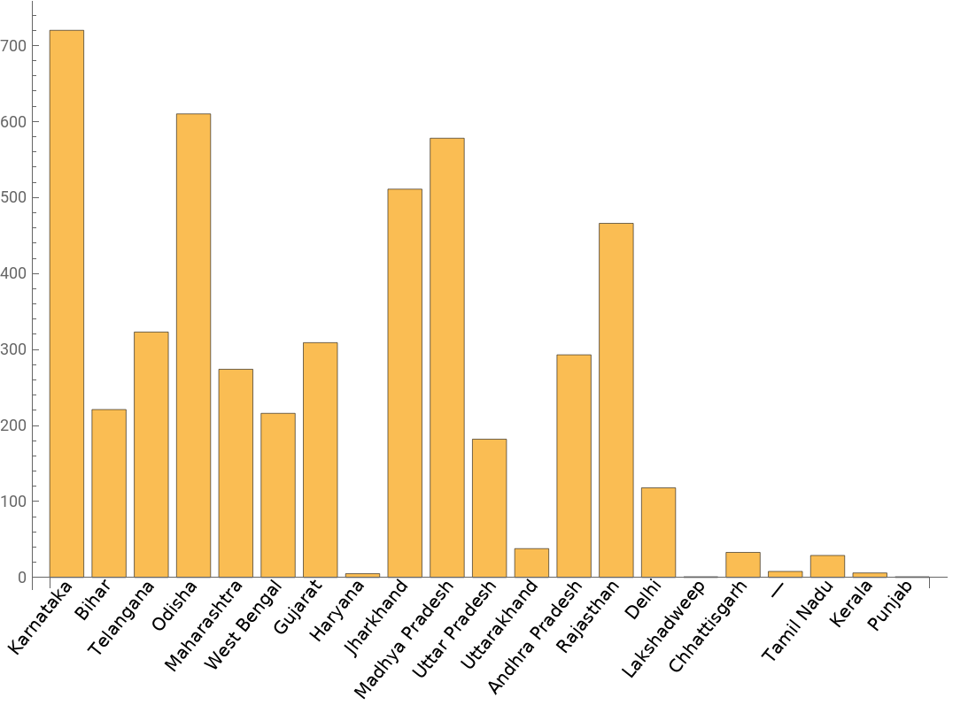
I started with some basic exploration of the datasets to get an idea of the population at hand. This was achieved through histograms, bar charts and pie charts. At first, I checked the state-wise count of the respondents. From the bar chart below we can observe that most of the respondents were from Karnataka, Odisha, Madhya Pradesh and Jharkhand. I followed this by finding out about the sex, caste and age group of the respondents.
In[]:=
labels={"Andaman and Nicobar Islands","Andhra Pradesh","Arunachal Pradesh","Assam","Bihar","Chandigarh","Chhattisgarh","Dadra and Nagar Haveli and Daman and Diu","Delhi","Goa","Gujarat","Haryana","Himachal Pradesh","Jammu and Kashmir","Jharkhand","Karnataka","Kerala","Ladakh","Lakshadweep","Madhya Pradesh","Maharashtra","Manipur","Meghalaya","Mizoram","Nagaland","Odisha","Puducherry","Punjab","Rajasthan","Sikkim","Tamil Nadu","Telangana","Tripura","Uttar Pradesh","Uttarakhand","West Bengal"};
In[]:=
val={1,2,3,4,5,6,7,8,9,10,11,12,13,14,15,16,17,18,19,20,21,22,23,24,25,26,27,28,29,30,31,32,33,34,35,36};
In[]:=
states=data1[All,"v111"]//Normal;Counts[states/.Thread[val->labels]];
In[]:=
keys=Keys[Counts[states/.Thread[val->labels]]];v=Values[Counts[states/.Thread[val->labels]]];
BarChart[v,ChartLabelsPlaced[keys,{{0.5,0},{0.9,1}},Rotate[#,(2/7)Pi]&]]
Out[]=
It is important to understand if the respondents went through any change in their work between the two rounds of survey.After making necessary changes of names and values, I compared the two columns of their respective datasets.
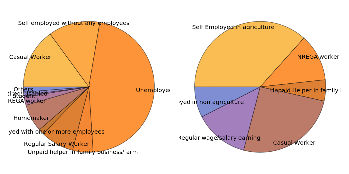
In the following piece of code I have taken “value” which counts the values of unique instances of different types of work that people did in February for the first round of interviews and I have taken “val” which performs the same function for the second dataset that covers the period of lockdown in India. “GraphicsRow” command is used to plot multiple charts in a row. From the charts below we can observe that while a major portion of respondents were unemployed, followed by self-employed just before the lockdown, during the lockdown a lot of them were employed in agriculture or became NREGA workers. This indicates that when covid cases had started rising rapidly the job scenario was also changing drastically.
In the following piece of code I have taken “value” which counts the values of unique instances of different types of work that people did in February for the first round of interviews and I have taken “val” which performs the same function for the second dataset that covers the period of lockdown in India. “GraphicsRow” command is used to plot multiple charts in a row. From the charts below we can observe that while a major portion of respondents were unemployed, followed by self-employed just before the lockdown, during the lockdown a lot of them were employed in agriculture or became NREGA workers. This indicates that when covid cases had started rising rapidly the job scenario was also changing drastically.
In[]:=
nonwork1=data1[All,"v301"]//Normal;nonwork2=data2[All,"q6041"]//Normal;
In[]:=
nonwork1=DeleteMissing[nonwork1];
In[]:=
priwork=Keys[Counts[nonwork1/.Thread[{1.0,2.0,3.0,4.0,4.5,5.0,6.0,7.0,8.0,9.0,10.0}->{"Self employed without any employees","Self employed with one or more employees","Regular Salary Worker","Casual Worker","NREGA worker","Unpaid helper in family business/farm","Unemployed","Student","Homemaker","Retired/Disabled","Others"}]]];value=Values[Counts[nonwork1/.Thread[{1.0,2.0,3.0,4.0,4.5,5.0,6.0,7.0,8.0,9.0,10.0}->{"Self employed without any employees","Self employed with one or more employees","Regular Salary Worker","Casual Worker","NREGA worker","Unpaid helper in family business/farm","Unemployed","Student","Homemaker","Retired/Disabled","Others"}]]];
In[]:=
nonwork2=DeleteMissing[nonwork2];
In[]:=
prk=Keys[Counts[nonwork2/.Thread[{1,2,3,4,5,6}->{"Self Employed in agriculture","Self Employed in non agriculture","Regular wage/salary earning","Casual Worker","NREGA worker","Unpaid Helper in family business/farm"}]]];val=Values[Counts[nonwork2/.Thread[{1,2,3,4,5,6}->{"Self Employed in agriculture","Self Employed in non agriculture","Regular wage/salary earning","Casual Worker","NREGA worker","Unpaid Helper in family business/farm"}]]];
ch1=PieChart[value,ChartLabelsPlaced[priwork,"RadialEdge"]];ch2=PieChart[val,ChartLabelsPlaced[prk,"RadialEdge"]];GraphicsRow[{ch1,ch2}]
Out[]=
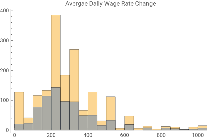
Next, I have plotted average daily wage rate for the respondents before and after lockdown. From the comparative histograms below and pie chart above, it is clear that there has been a significant dip in their earnings because a lot of salaried employees had to take up other forms of employment.
(*v204-204.WhatwastheaverageDAILYwagerateatwhichyouwereworkinginthemonthofFebruary?q409-Onaverage,whatwasyourdailywagerateduringthisperiod?*)
wage2=data2[All,"q409"]//Normal;wage1=data1[All,"v204"]//Normal;Histogram[{wage1,wage2},PlotLabel"Avergae Daily Wage Rate Change",ChartLegends{"Round1","Round2"}]
Out[]=


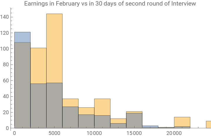
The second comparison below shows us the difference in their earnings from their business/enterprise. While there appears to be an increase in for a lower amount, considering that a lot of the respondents had taken up agricultural work, there has been an overall dip in their earnings.
(*v206-HowmuchdidyouearninyourbusinessinthemonthofFebruary?q402-Whatwasyourtotalearningsfromtheenterpriseforthelast30daysofinterview?*)
earn2=data2[All,"q402"]//Normal;earn1=data1[All,"v206"]//Normal;Histogram[{earn1,earn2},PlotLabel"Earnings in February vs in 30 days of second round of Interview",ChartLegends{"Round1","Round2"}]
Out[]=


Comparing change in data
Comparing change in data
Here I have taken some important factors during both rounds of interviews to observe the change in behaviour of the population. Considering that round 2 had about half of the original population, hence a lot of it included missing values and the data is nominal therefore, I have used DeleteMissing[] to treat the missing values. Furthermore, I have used MatrixPlot function which gives a visual representation of the values of elements in a matrix.
I have taken the following columns from Round 1 dataset:
(*v510-Doyouthinkyouwillreturntoyourplaceofworkafterthelockdownislifted?v511.Doyouthinkyouwillcontinueinyourplaceofworkafterthelockdownislifted?*)
Here I have used the MatrixPlot function to plot the values which were sent as lists. ArrayPlot function can also be used however it may not be able to distinguish between large numbers of different values.
From the Round 2 dataset I have used the following columns and again plotted the using MatrixPlot function:
Finally, I have plotted them side by side to get a comparative picture of people’s responses to similar questions in each round. From the graphs it can be observed that the responses for food consumption and change of residence/ place of work has drastically changed. This is an affirmation of the fact that migration during the lockdown or in the initial stages of the lockdown has affected a lot of people and due to change in income and livelihood one of the most affected areas can be considered food consumption.
In the next part of the project, I have tried to observe sentiments surrounding COVID and unemployment through twitter data.
In the next part of the project, I have tried to observe sentiments surrounding COVID and unemployment through twitter data.
Sentiment analysis of COVID -19 and unemployment tweets
Sentiment analysis of COVID -19 and unemployment tweets
In this section, I have tried to find sentiment behind tweets related to COVID-19 and unemployment in India. To that end, I have used trigrams of popular phrases in the initial months of COVID and recent tweets pertaining to these topics. While the trigrams have been extracted from tweets during the start of the pandemic so they are not exclusively covid related, the tweets that have been downloaded using Wolfram’s TweetSearch function are a direct response to the query “covid” and “unemployment”.
Trigrams are a special case of the n-gram where n is 3; in other words it's a figure made up of three whole or broken lines. They are often used in natural language processing for performing statistical analysis of texts and in cryptography for control and use of ciphers and codes. I downloaded a dataset of top 1000 trigrams from all the tweets and retweets related to COVID-19 chatter in 2021.
Finding sentiment in popular trigrams
Finding sentiment in popular trigrams
Wolfram Language has an inbuilt classifier to categorize words of sentences into "Neutral", "Positive", "Negative", and "Indeterminate" categories. Here, I have stored the trigrams into a list which is then sent to the Classify function which treats each trigram as a sentence and determines the sentiment. Next, we have counted the occurence of each sentiment type and created a bar chart to depict the results. From the results we can see that it was more positive than negative but this is mostly because the dataset consists of isolated trigrams where the context of the whole tweet may not be clear.
Next, I have tried to analyse the sentiments of COVID-19 tweets from recent times. The first thing to be done is to connect to twitter. This can be done by creating a variable twitter, and using ServiceConnect to set up a new connection from Mathematica to your twitter account.
After that, the twitter API needs to be activated to scrape tweets from its website. Next step is to focus on gathering the data. To this end, I created a variable tweets, and into it, inputted the query, location, radius of the area I was looking for results in, and the language of the tweets which I wanted to select. It is necessary to specify the language since the Classify function to be used to get the sentiment of the tweet is best used on tweets which were already in English.
The TweetSearch function automatically filters for the most recent tweets, meaning that using said function wouldn’t allow us to get covid sentiment from specific time periods so it limits us from gathering data over time to look at how sentiment about coronavirus has changed. Another problem is that a lot of people tweet in regional languages which automatically get filtered out.
Sentiment of recent COVID-19 tweets
Sentiment of recent COVID-19 tweets
Any text of the tweets extracted from this data contains several entities that are of no use to our programs so it is necessary to remove them. I cleaned the data to remove hashtags, URLs and "@" signs form the tweet texts by creating a function with detects "#", "https://" and "@" and removes them from the text.
Some exploratory statistics of the tweets:
To get a general idea of the kind of tweets I had scraped, I perfomed the following functions. This was achieved by getting the favourite count and retweet count and creating a function to find the most popular tweets wherein I stored the highest number of favourites and retweets in different variables and equated the respective FavouriteCount and RetweetCount of each tweet to get the one which had bigger value.
To get a general idea of the kind of tweets I had scraped, I perfomed the following functions. This was achieved by getting the favourite count and retweet count and creating a function to find the most popular tweets wherein I stored the highest number of favourites and retweets in different variables and equated the respective FavouriteCount and RetweetCount of each tweet to get the one which had bigger value.
Furthermore, we can visualise the data into a WordCloud of most popular terms in the COVID chatter. It must be noted that this WordCloud consists of tweets which have been cleaned, i.e, hashtags, URLs and "@" removed using the clean function above and stopwords removed using Wolfram's built-in "DeleteStopwords" function.
After that I created functions to filter tweets to remove further unnecessary words, removing profanities and cases of same words. Further, I created a function which takes the Processed tweets and then arranges them according to signficance of frequency of occurence. In other words, this function creates the set of words occuring from most number of times to least number of times and then we extract the top ten terms from there. I displayed this as a pie chart to show percent of occurrence of popular terms.
Some of the top terms can be counted as neutral but it is hard to tell if for the overall data the sentiment is more negative than it is positive. This is checked by classifying the sentiment of the tweets using the Classify function.
Pie Chart of sentiments of covid related tweets
While the major sentiment remains neutral, we can see that positive covers more area in the piechart than negative which can be attributed to the fact that a large portion of the adult Indian population is now vaccinated, therefore one can say that the initial shock has worn off.
Sentiment of unemployment related tweets in India
Sentiment of unemployment related tweets in India
I downloaded unemployment related tweets using TweetSearch function once again.
For this section, I performed similar steps as the first half. I cleaned the data to remove hashtags, URLs and "@" and then I proceeded to find out favourite and retweet counts and most favourite or retweeted tweets.
Then I visualised the data into a WordCloud of most popular terms in the unemployment chatter. It must be noted that this WordCloud consists of tweets which have been cleaned, i.e, hashtags and "@" removed using the clean function above and stopwords removed using Wolfram's built-in "DeleteStopwords" function.
I recreated the filter function to remove unnecessary words, profanities and duplicate cases. Next using the same methodology as the previous section, I gathered the most frequent terms and created a pie chart to show percentage of occurence of most popular terms.
Pie chart to show sentiment of the tweets
In this pie chart we can see that even though the sentiment was majorly neutral, negative sentiment prevailed over positive.
Comparison of sentiments between the two categories
Comparison of sentiments between the two categories
This comparison shows the twitter chatter recently has been more negative with respect to unemployment than covid.
Conclusion
Conclusion
While the COVID cases are still rising daily, this data is proof that people’s lives have not come to a complete stand still just because of the lockdown. Although the data available for the second round did not have as many responses as the first round, we can observe some changes in the state of work. This further implies changes in living standards which were impacted by death and illness besides job status. Through this project we are able to observe if there is any change in factors from before lockdown and after lockdown. This project has thrown some light on the fact that average wage rate for salaried employees decreased overall, income for people with businesses also changed and there was drastic change in the responses of people when questioned about where they where located before lockdown and further into the lockdown. This implies that people had to change residences or place of work. It can also be observed that people’s food consumption behaviour was also quite affected. From here further research can be carried on to find if any dependance has changed over an extended period of time and how exactly the state of employment has affected the lives of these people.
From the twitter sentiment analysis we can draw inferences about the trending topics surrounding the COVID chatter. Clearly, while the overall sentiment seems to be neutral people of India are not as bitter about COVID as they are about the state of employment. However, this twitter data has been acquired dynamically which means that it only shows very recent data and limited number of tweets therefore it would be incorrect to generalise it for a larger period of time.
In conclusion, the pandemic has clearly touched every aspect of our lives and changed them, especially in the case of jobs and livelihood.
Keywords
Keywords
◼
covid
◼
unemployment
◼
correlation
◼
sentiment analysis
◼
twitter
Acknowledgment
Acknowledgment
I would like to take this opportunity to extend my gratitude to my mentor Sotiris Michos for constantly guiding me every step of the way while making this project. Sotiris' guidance not only helped me make this project a better one than what I had in mind but also helped me learn a lot of new things. Furthermore, I would like to thank all the TAs involved in the Winter School Programme for always promptly coming to my aid whenever I required and understanding my necessities. Lastly, I would like to thank the programme co-coordinators for creating a wonderful opportunity for people like myself because this has been an incredible learning opportunity and it gave me a platform to discuss and exchange ideas with such vastly talented and resourceful people.
References
References
◼
Due to the relevance of the COVID-19 global pandemic, a dataset of tweets acquired from the Twitter Stream related to COVID-19 chatter has been curated and released. Since its first release, additional data from new collaborators have been added. Dedicated data gathering started from March 11th yielding over 4 million tweets a day. Banda, Juan M., Tekumalla, Ramya, Wang, Guanyu, Yu, Jingyuan, Liu, Tuo, Ding, Yuning, Artemova, Katya, Tutubalina, Elena, & Chowell, Gerardo. (2021). A large-scale COVID-19 Twitter chatter dataset for open scientific research - an international collaboration (Version 70) [Data set]. Trigrams downloaded from https://zenodo.org/record/5090588#.YdR3SmhBw2w
◼
In April and May 2020, Azim Premji University partnered with ten Civil Society Organisations to do a phone survey (Round 1) of nearly 5,000 workers across several major states on the impact of the lockdown on livelihoods. A subsequent round (Round 2) was conducted between October and December 2020 to gauge the extent of economic recovery. Of the nearly 5,000 workers interviewed during the lockdown, we managed to reach 2,778 respondents in Round 2. Survey data downloaded from https://cse.azimpremjiuniversity.edu.in/cse-surveys/covid19-livelihoods-phone-survey/
Round 1 and Round 2 data along with Codebook available in Google Drive under this link.
Round 1 and Round 2 data along with Codebook available in Google Drive under this link.