Wolfram Cloud Document

We give a guided tour into the method of support vector regression. We start from the primal optimization problem and then proceed to the dual problem. We explain the use of kernels. A program is written for the method of support vector regression. Cross-validation is used to estimate the unknown parameters. Two example data sets are fitted by four methods: polynomial regression, polynomial support vector regression, Gaussian support vector regression, and local regression.

Introduction

With Mathematica, we can apply many regression methods. Examples are

• linear regression: Fit, LinearModelFit, GeneralizedLinearModelFit,
• nonlinear regression:FindFit, NonlinearModelFit,
• logistic and probit regression: LogitModelFit, ProbitModelFit.

We also have several methods provided by Predict, a function related with machine learning. These methods are currently as follows:
“DecisionTree”, “GradientBoostedTrees”, “LinearRegression”, “NearestNeighbors”, “NeuralNetwork”, “RandomForest”, and “GaussianProcess”.

One of the methods related with machine learning is support vector regression, for which we currently do not have a built-in function. In this notebook, we give a short introduction to and a program for the method of support vector regression. We also compare it with polynomial regression and local regression by analysing two numerical examples, one two-dimensional and one three-dimensional.

The fitting methods have various parameters that have to be chosen in some way. For example, in polynomial regression we have to choose the degree of the polynomial. One way is to use a subjective decision: the fit is calculated by using several values of the parameters and the parameters are chose that, subjectively, seem to be good. Another way is to use a mathematical criterion like the root mean square error (RMSE). We resort to this criterion, by applying the well-known method of cross-validation.

This notebook is based on Ruskeepää (2017) which, in addition to introducing support vector regression and using polynomial and local regression, also applies the methods provided by the Predict function and compares all the eight prediction methods by applying them to eleven data sets.

For a literature review of the method of support vector regression, see, for example, Smola and Schölkopf (2004). A few other references could be Vapnik (1995), Cristianini and Shawe-Taylor (2000), and Hastie, Tibshirani, and Friedman (2013). For support vector machines with Mathematica, see Paláncz (2004), Paláncz, Volgyesi, and Popper (2005), and Nilsson, Björkegre, and Tegnér (2006).

1 The Primal Optimization Problem

1.1 A First Try

Consider the data

T={(

),…,(

)}

; we call this data set the training data. The

’s are

-vectors. We would like to fit a linear function of the form

f(x)=w·x+b

to the data. Here,

is a constant and

w·x

is the inner product of a constant vector

w=(

,…,

)

and the vector of variables

x=(

,…,

)

, that is,

w·x=

∑

j=1

. In usual least-squares regression, we minimize the sum

∑

i=1

(

-f(

))

, that is, the sum of the squares of the fitting errors, by finding the best values of

and

. Now, we try a different approach.

First, we require that, for all

)

differs from

by at most a given amount ϵ. So, we should have

w·

+b≤

+ϵ,

w·

+b≥

-ϵ,

i=1,…,m

. Hence, we do not care about fitting errors at all as long as they are smaller than ϵ; however, an error larger than ϵ is not accepted at all. Second, we ask for a flat

f(x)

, which means that

w

should be minimized.

As an example, consider the following data:

In[]:=

SeedRandom[1];data=Table[{x,0.3x+1+RandomVariate[NormalDistribution[0,0.25]]},{x,0,5,0.2}]

Out[]=

{{0.,1.12142},{0.2,1.12547},{0.4,1.50607},{0.6,1.21267},{0.8,1.13581},{1.,1.29628},{1.2,1.36516},{1.4,1.44444},{1.6,1.39308},{1.8,1.64208},{2.,1.7799},{2.2,1.56909},{2.4,1.8659},{2.6,1.46786},{2.8,1.97954},{3.,2.00759},{3.2,1.65621},{3.4,2.19126},{3.6,1.74887},{3.8,2.09606},{4.,2.18573},{4.2,1.89467},{4.4,1.72249},{4.6,2.43666},{4.8,2.18554},{5.,2.67924}}

In[]:=

m=Length[data]

Out[]=

In[]:=

p1=ListPlot[data,PlotStyle->Black]

Out[]=

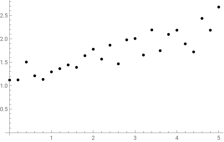
Let us formulate the optimization problem mentioned above. We have

n=1

and

m=26

. Let us choose

ϵ=0.6

In[]:=

n=1;ϵ=0.6;

From the data, we separate the independent variable

and the dependent variable

In[]:=

xx=Most/@data

{{0.},{0.2},{0.4},{0.6},{0.8},{1.},{1.2},{1.4},{1.6},{1.8},{2.},{2.2},{2.4},{2.6},{2.8},{3.},{3.2},{3.4},{3.6},{3.8},{4.},{4.2},{4.4},{4.6},{4.8},{5.}}

In[]:=

yy=Last/@data

Out[]=

{1.12142,1.12547,1.50607,1.21267,1.13581,1.29628,1.36516,1.44444,1.39308,1.64208,1.7799,1.56909,1.8659,1.46786,1.97954,2.00759,1.65621,2.19126,1.74887,2.09606,2.18573,1.89467,1.72249,2.43666,2.18554,2.67924}

We form the vectors

and

In[]:=

W=Array[

&,n]

Out[]=

{

}

In[]:=

X=Array[

&,n]

Out[]=

{

}

We form the constraints:

In[]:=

cons1=Table[W.xx[[i]]+b≤yy[[i]]+ϵ,{i,m}]

Out[]=

{0.+b≤1.72142,b+0.2

≤1.72547,b+0.4

≤2.10607,b+0.6

≤1.81267,b+0.8

≤1.73581,b+1.

≤1.89628,b+1.2

≤1.96516,b+1.4

≤2.04444,b+1.6

≤1.99308,b+1.8

≤2.24208,b+2.

≤2.3799,b+2.2

≤2.16909,b+2.4

≤2.4659,b+2.6

≤2.06786,b+2.8

≤2.57954,b+3.

≤2.60759,b+3.2

≤2.25621,b+3.4

≤2.79126,b+3.6

≤2.34887,b+3.8

≤2.69606,b+4.

≤2.78573,b+4.2

≤2.49467,b+4.4

≤2.32249,b+4.6

≤3.03666,b+4.8

≤2.78554,b+5.

≤3.27924}

In[]:=

cons2=Table[W.xx[[i]]+b≥yy[[i]]-ϵ,{i,m}]

Out[]=

{0.+b≥0.52142,b+0.2

≥0.52547,b+0.4

≥0.906075,b+0.6

≥0.612675,b+0.8

≥0.535811,b+1.

≥0.696283,b+1.2

≥0.765163,b+1.4

≥0.844441,b+1.6

≥0.793085,b+1.8

≥1.04208,b+2.

≥1.1799,b+2.2

≥0.969092,b+2.4

≥1.2659,b+2.6

≥0.867858,b+2.8

≥1.37954,b+3.

≥1.40759,b+3.2

≥1.05621,b+3.4

≥1.59126,b+3.6

≥1.14887,b+3.8

≥1.49606,b+4.

≥1.58573,b+4.2

≥1.29467,b+4.4

≥1.12249,b+4.6

≥1.83666,b+4.8

≥1.58554,b+5.

≥2.07924}

The objective function is

In[]:=

obj=0.5Total[

]

Out[]=

0.5

The variables are

In[]:=

vars=Join[W,{b}]

Out[]=

{

,b}

We then solve the optimization problem:

In[]:=

{val,sol}=FindMinimum[{obj,cons1,cons2},vars]

Out[]=

{0.00334302,{

0.0817682,b1.6704}}

The minimum value of the objective function is 0.0033… Here is the resulting line:

In[]:=

f=W.X+b/.sol

Out[]=

1.6704+0.0817682

We also calculate the margins that are at the distance ϵ from the line:

In[]:=

marg1=W.X+b+ϵ/.sol

Out[]=

2.2704+0.0817682

In[]:=

marg2=W.X+b-ϵ/.sol

Out[]=

1.0704+0.0817682

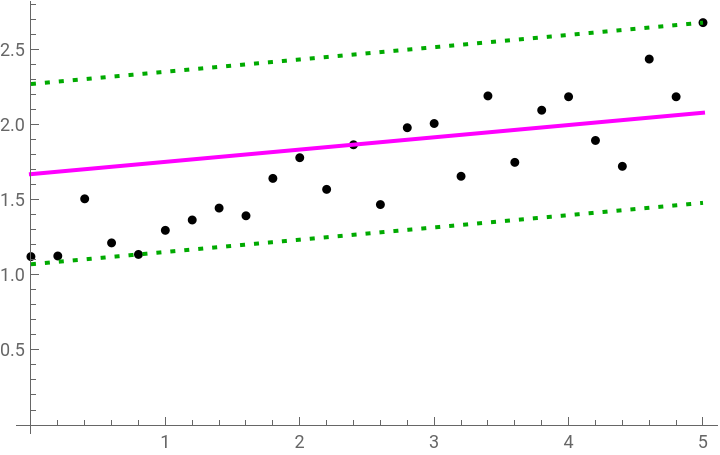
We plot the lines together with the data. The fit is magenta and the margins are green:

In[]:=

Show[p1,Plot[f,{

,0,5},PlotStyleMagenta],Plot[{marg1,marg2},{

,0,5},PlotStyle{{Dashing[Small],Darker[Green]}}]]

Out[]=

The fitting errors are as follows:

In[]:=

err=yy-(f/.

#[[1]]&/@xx)

Out[]=

{-0.548977,-0.56128,-0.19703,-0.506783,-0.6,-0.455882,-0.403356,-0.340432,-0.408141,-0.175505,-0.0540367,-0.281194,-0.000745431,-0.415136,0.0801895,0.0918869,-0.275848,0.24285,-0.215887,0.114947,0.188258,-0.119155,-0.307687,0.390134,0.122653,0.6}

In[]:=

ListLinePlot[err,MeshAll,Epilog{Thick,Dashing[Small],Darker[Green],Line[{{0,ϵ},{26,ϵ}}],Line[{{0,-ϵ},{26,-ϵ}}]}]

Out[]=

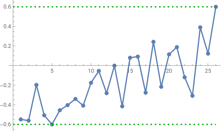
We see that all the errors are, indeed, smaller that

ϵ=0.6

but otherwise the solution (the magenta line in the earlier plot) does not look good: the slope should be larger. The solution would be somewhat better by choosing a smaller ϵ, but ϵ cannot be much smaller; indeed, the smallest value is approximately 0.41. If ϵ is smaller, no solution exists. Thus, we have to develop our model further.

1.2 The Primal Optimization Problem

We now make the constraints somewhat less stringent, or soft, by allowing a violation of the constraints:

The constraints are as follows:

The objective function is

The variables are

We then solve the optimization problem:

Many variables are almost zero. We make them zero:

We plot the resulting line and margins together with the data:

The errors are as follows:

Note that objective function of the primal problem is relatively simple but we have lots of constraints. When we, in Section 2.1, derive the so-called dual problem, we observe that it has a long objective function but, besides the non-negativity constraints, only one equality constraint.

1.3 The Quadratic ϵ-Insensitive Loss Function

Because the loss is zero if the error is at most ϵ, the loss function is called to be ϵ-insensitive. Because the loss is quadratic if the error is at least ϵ, this loss function is called a quadratic ϵ-insensitive loss function.

1.4 Importance of the Support Vectors

Let us demonstrate the support vectors with the preceding example. The positive variables were as follows:

We only take these data points:

Define the variables:

Define the constraints and the objective function:

The solution is

This is exactly the same result we got in Section 1.2. We get the same line:

2 The Dual Optimization Problem

2.1 Derivation of the Dual Problem

In Section 1.2, we arrived at the following primal optimization problem:

We could solve the fitting problem by solving this optimization problem. However, we continue the development of support vector regression by transforming this problem into another form called the dual optimization problem. The advantage of this form will be seen in Section 3.1 where we introduce the so-called kernels; these functions simplify the dual problem considerably.

This can be written as

Thus,

So, we know that

In addition, we have

The Lagrangian then becomes to the form

So,

Recall that, in the primal problem, the objective function was relatively simple but we had lots of constraints. In the dual problem, we observe that it has a long objective function but, besides the non-negativity constraints, only one equality constraint.

2.2 Solving the Primal Problem

The regression hyperplane is then

5 Simple Examples

5.1 The Simple Example Revisited

As an example, we solve the example of Section 1.1:

The solution is as follows:

In Section 1.2 we got the same solution by solving the primal problem, and, in Section 2.3, we also got the same solution by first solving the dual problem.

With these settings, the resulting regression curve follows the data quite closely and we have lots of support vectors. With a larger ϵ, we have fewer support vectors; this causes, in our example, more curvature:

5.2 Some Limiting Cases

Recall the primal optimization problem: minimize

subject to

The least-squares fit is

Second, here is a least-squares fit with the basis that contains the Gaussian kernel at the same points as above:

When we plot the two fits, we see that they are almost the same:

The least-squares fit (the brown curve) still follows the data too closely but the support vector fit (the blue curve) is a good approximation to the data.

5.3 Another Simple Example

Consider the chemical data given in Ivanciuc (2007, s. 298):

The same holds for a larger ϵ:

7 Temperature against Ozone: Four Methods

7.1 Polynomial Regression

7.1.1 Introduction

To familiarize with the fitting problem, consider the ozone and temperature data introduced in Section 6.1 and calculate a fourth-degree polynomial fit:

The fit together with the data is as follows:

A plot of the residuals is as follows:

It can also be calculated as follows:

This plot contains a cubic fit to the residuals. The fit should be close to zero. In our example, the fit is reasonable near to zero. The root mean square of the residuals should be small; in our example, it is 6.04171. The RMSE can be used to select a good model from among several candidates.

7.1.2 Calculating the Best Fit

The fits do not differ a lot, except the linear fit.

The program gives two results: the smallest RMSE (RMSE[1]) and a plot (g[1]) of all the RMSE computed. The smallest RMSE is

Here are all the RMSE’s we calculated:

We see that, according to cross-validation, a second-degree fit is the best with an RMSE of 6.28495. We get the following fit:

We show this fit together with the data (see Section 4.4):

The comparison plot is as follows if we use the cross-validation method (see Section 4.4):

The residuals are

7.2 Polynomial Support Vector Regression

7.2.1 Exploring the Parameters

The best value of ϵ is 2. The corresponding RMSE is 6.266. We then do a second search. We now use ϵ = 2 and try, for C, the values 700, 710, 720, and 730:

The best value of ϵ is 1.95. We do still a closer look and investigate the values 1.95, 1.96, and 1.97:

The best value of ϵ is 1.96. The corresponding RMSE is

7.2.2 Calculating the Best Fit

We got the following parameters:

So, we get the following fit:

In the expanded form, the fit is as follows:

With polynomial regression we got the fit

These two fits differ somewhat:

The upper, blue curve is the polynomial fit and the lower, orange curve the fit given by polynomial support vectors.

The next plot only shows the data and the fit:

Recall that with polynomial regression we got the RMSE of 6.28495. This is a little larger than the RMSE of 6.03817 we got by polynomial support vector regression with a second-order polynomial kernel.

7.3 Gaussian Support Vector Regression

7.3.1 Exploring the Parameters

7.3.2 Finding the Optimal Parameters

and then generate four random points, the first of them being the given point:

This method is used by the optimizeSupportVectorRegression program.

The computation took approximately 3 minutes. The smallest value of the RMSE is 6.26438. Note that with the simple search we arrived at the RMSE of 6.26493 which is already very near to the smallest value. Also, the values of the parameters found with optimization are quite near to the starting values.

From the plot we can see that the RMSE, as a function of σ and C, has quite a flat valley: we can see a long area of near-optimal points. This means that we can get almost the same RMSE with quite different values of the parameters σ and C.

7.4 Local Regression

7.4.3 Examples

This fit looks quite good. We also try as few local polynomials as 5:

Now we only use 5 local polynomials:

7.4.3 Exploring the Parameters

In local regression, we can apply first- and second-order local polynomials. First, we consider first-order local polynomials. Below are the RMSE’s by using various numbers of first-degree local polynomials and various values of the smoothing constant α .

We take a closer look:

7.4.4 Calculating the Best Fit

We have arrived at the following fit:

For comparison, here is the best fit by using second-degree local polynomials:

8 Temperature against Wind and Radiation: Four Methods

8.1 The Data

The continue with the environmental data considered in Section 6:

The data has 111 observations, each of which contains the value of ozone, radiation, temperature, and wind. First, we separate the components:

Now, we would like to analyze temperature against wind and radiation:

In three dimensions, the data looks as follows:

As wind increases, the temperature has a descending pattern.

Here are the five training data sets:

Below are the five validation data sets:

8.2 Polynomial Regression

Here are then the four fits:

They look as follows:

We see that the quadratic fit is the best. Here is the fit:

We also show the fit from another viewpoint to show that we, of course, also have data points below the surface:

The comparison and residual plots are as follows:

8.3 Polynomial Support Vector Regression

The computation took approximately 11 minutes. The RMSE = 7.61938 is better than the RMSE 7.6672 with polynomial regression. We did not get a better RMSE by exploring values of ϵ. Applying true optimization to find the optimal C and ϵ needs very long computation time we will not do that. Instead we use the values C = 31 and ϵ = 1 we got with the simple explorations:

The fit looks as follows:

The comparison and residual plots are as follows:

8.5 Local Regression

First, we consider first-order local polynomials. Below are the RMSE’s by using various numbers of first-degree local polynomial surfaces and various values of the smoothing constant α (the computation time is approximately three minutes).

We show a closer view:

References

◼

Cleveland, W. S. (1993). Visualizing Data. Hobart Press, Summit, NJ.

◼

Cristianini, N., and J. Shawe-Taylor (2000): An Introduction to Support Vector Machines and Other Kernel-Based Learning Methods. Cambridge University Press, Cambridge.

◼

Hastie, T., R. Tibshirani, and J. Friedman (2013): The Elements of Statistical Learning: Data Mining, Inference, and Prediction, 7th corrected printing. Springer, New York.

◼

Ivanciuc, O. (2007): Applications of support vector machines in chemistry. In K. B. Lipkowitz and T. R. Cundari, Eds.: Reviews in Computational Chemistry, Vol. 23, p. 291–400, Wiley-VCH, Weinheim.

◼

Nilsson, R., J. Björkegre, and J. Tegnér (2006): A flexible implementation for support vector machines. The Mathematica Journal, Vol. 10, Issue 1.

◼

Paláncz, B. (2004): Support vector regression via Mathematica. Wolfram Library Archive.

◼

Paláncz, B., L. Volgyesi, and G. Popper (2005): Support vector regression via Mathematica. Periodica Polytechnica Civil Engineering, Vol. 49(1).

◼

Ruskeepää, H. (2009): Mathematica Navigator: Mathematics, Statistics, and Graphics, Third Ed. Elsevier Academic Press, Burlington, MA.

◼

Ruskeepää, H . (2017): Support vector regression and other prediction methods: A competition with Mathematica. Wolfram Library Archive.

◼

Smola, A. J., and B. Schölkopf (2004): A tutorial on support vector regression. Statistics and Computing, Vol. 14, p. 199–222.

◼

Vapnik, V. (1995): The Nature of Statistical Learning Theory. Springer, New York.

CITE THIS NOTEBOOK

An Introduction to Support Vector Regression
by Heikki Ruskeepää
Wolfram Community, STAFF PICKS, December 13, 2023
https://community.wolfram.com/groups/-/m/t/3083213