This notebook series is designed to introduce selected dynamic economic models to both advanced undergraduate and graduate students. Economists have relied on a series of economic models to better understand the otherwise highly complex causal relationship among many economic variables. Dynamic economic models set up by systems of either difference or differential equations are particularly useful in tracing the change in the quantity of unknown economic variables (e.g., the capital stock, demand for labor, aggregate output, etc.) and their interactions over time.
This notebook series aims to help students better understand the depth, usefulness, and limitations of major existing micro and macroeconomic models by demonstrating how we can use Wolfram Mathematica to replicate and reconstruct the core ideas and find dynamic solution of the model.
The model introduced in this notebook series include, among others, (1) the cobweb model of the quantity and price adjustment, (2) Keynes’s aggregate demand model, (3) Hicks’s ISLM model, (4) Samuelson’s investment accelerator model, (5) Kalecki’s investment delay model, (6) the predator-prey interaction model, (7) the epidemic model, (8) Ricardo’s three dimensional business cycle model, (9) Marx-Goodwin business cycle and growth model, (10) Smith’s and Ricardo’s growth model, (11) the Harrod-Domar growth model, (12) the Solow growth model, (13) the RBC model, (14) Romer’s new growth model, and (15) the circuit of capital model.
Introduction
Introduction
In Principles of Political Economy and Taxation, David Ricardo provides an interesting analysis of the effect of the capital stock accumulation in the agricultural sector. Ricardo proposes the idea that the accumulation of the capital stock in agriculture tends to increase both demand for labor and nominal wages on the one hand and the increase in prices of foods and ground rent that capitalist farmers pay to owners of land on the other. This rising differential rent and nominal wages soon become an obstacle to a further accumulation of the capital stock in the same sector because a greater portion of gross profits of capitalist farmers will be paid to landowners and wage laborers. The initial predator-prey relation formed between landowners and capitalist farmers becomes more complicated when it instigates the dynamic interactions and interest conflicts between capitalist farmers and wage laborers in the same sector.
In Ricardo, the ground rent accruing to landowners inevitably rises as the capital stock accumulation proceeds because there emerges a greater demand for cultivating land for producing agricultural products. Since arable land is limited in quantity and has a differential fertility, the rising demand for agricultural products necessarily induces the rising rent that capitalist farmers have to pay to the owner of land. Nominal wages for laborers also tend to rise as the capital stock accumulates further in the agricultural sector because agricultural capitalists compete with one another to hire more agricultural laborers. In consequence, and especially in the absence of any meaningful offsetting mechanisms (such as the importation of cheaper foods from abroad or as suppressing nominal wages by extra economic forces), any further accumulation of the capital stock will be impeded as the profit of capital falls in the face of rising rent and labor cost (Ricardo 1996: 53-56, 65-67, 68-71, 76-88).
This idea of the long-run tendency of the average rate of profit to fall in the agricultural sector can be modeled by defining three differential equations with appropriate parameters. From a mathematical point of view, Ricardo’s ‘income-distribution-led growth dynamics’ involves the three stocks linked with the three corresponding parameters, which is similar to the Lorenz equation (Lorenz 1963) and Herbert, Elsworth and Telling (1956)’s chemostat model of complexity. This note shows how we can set up a model to replicate Ricardo’s core messages.
Specifications of variables and parameters
Specifications of variables and parameters
Let us use rT to denote total rent income accruing to landowners, wL total nominal wage income paid to wage laborers, and πK total gross profit income capitalist farmers earn. Both total rent and wage income rise as gross profit income increases. But the profit income begins to fall as both rent and wage income increase and reach a certain critical threshold.
If we redefine x ≡ rT, y ≡ wL, and z ≡ πK, we can write this dynamic and interdependent relationships among the three income variables in the following way:
x
y
z
This system consists of three first-order, homogeneous, autonomous, but non-linear differential equations, which requires some additional qualitative analyses.
Steady state values
Steady state values
The steady state points of this system can be found by setting all the differential terms equal to zero. If we set = = = 0 and solve the resulting three equations simultaneously, we get the following three steady state values:
x
y
z
In[]:=
Clear[a,b,c,x,y,z,α,β,γ,δ,f,g,h];f[x_,y_,z_]:=-ax+αxz;g[x_,y_,z_]:=-by+βyz;h[x_,y_,z_]:=cz-γxz-δyz;Solve[{f[x,y,z]==0,g[x,y,z]==0,h[x,y,z]==0},{x,y,z}]
Out[]=
x0,y,z,x,y0,z,{x0,y0,z0}
c
δ
b
β
c
γ
a
α
The stability of the system
The stability of the system
The stability of this system depends on the sign of trace and determinant of the Jacobian coefficient matrix evaluated at and near the three steady state values.
The Jacobian coefficient matrix can be found by:
In[]:=
J=
D[f[x,y,z],x] | D[f[x,y,z],y] | D[f[x,y,z],z] |
D[g[x,y,z],x] | D[g[x,y,z],y] | D[g[x,y,z],z] |
D[h[x,y,z],x] | D[h[x,y,z],y] | D[h[x,y,z],z] |
Out[]=
{{-a+zα,0,xα},{0,-b+zβ,yβ},{-zγ,-zδ,c-xγ-yδ}}
In[]:=
{{-a+zα,0,xα},{0,-b+zβ,yβ},{-zγ,-zδ,c-xγ-yδ}}//MatrixForm
Out[]//MatrixForm=
-a+zα | 0 | xα |
0 | -b+zβ | yβ |
-zγ | -zδ | c-xγ-yδ |
If we evaluate this Jacobian matrix at the three steady state values, we get:
In[]:=
J/.{x->0,y->0,z->0}//MatrixFormJ/.x0,y,z//MatrixFormJ/.x,y0,z//MatrixForm
c
δ
b
β
c
γ
a
α
Out[]//MatrixForm=
-a | 0 | 0 |
0 | -b | 0 |
0 | 0 | c |
Out[]//MatrixForm=
-a+ bα β | 0 | 0 |
0 | 0 | cβ δ |
- bγ β | - bδ β | 0 |
Out[]//MatrixForm=
0 | 0 | cα γ |
0 | -b+ aβ α | 0 |
- aγ α | - aδ α | 0 |
Now we can find the trace and determinant of these three matrices.
In[]:=
Tr
Det
-a | 0 | 0 |
0 | -b | 0 |
0 | 0 | c |
-a | 0 | 0 |
0 | -b | 0 |
0 | 0 | c |
Out[]=
-a-b+c
Out[]=
abc
In[]:=
Tr
Det
-a+ bα β | 0 | 0 |
0 | 0 | cβ δ |
- bγ β | - bδ β | 0 |
-a+ bα β | 0 | 0 |
0 | 0 | cβ δ |
- bγ β | - bδ β | 0 |
Out[]=
-a+
bα
β
Out[]=
-abc+cα
2
b
β
In[]:=
Tr
Det
0 | 0 | cα γ |
0 | -b+ aβ α | 0 |
- aγ α | - aδ α | 0 |
0 | 0 | cα γ |
0 | -b+ aβ α | 0 |
- aγ α | - aδ α | 0 |
Out[]=
-b+
aβ
α
Out[]=
-abc+cβ
2
a
α
At this level, unfortunately, we cannot directly determine the sign of either trace or determinant, and, therefore, we cannot draw any definite conclusion of qualitative behaviors of this system. Depending on the size and sign of both trace and determinant of the three Jacobian matrices evaluated at the three steady state values, one can anticipate that the model either converge to or diverge away from a particulate steady state value. It is also possible that the system solution constantly oscillate around any of the three steady state values.
A static visualization of the solution curves
A static visualization of the solution curves
One possible analytical solution to this system can be found by assuming that nominal wages are brought down to their subsistence level, thereby transforming the variable y no longer binding as an independent variable. In this case, the entire system is reduced to a system of two differential equations that is similar to a classic predator-prey relation between rent and profit income:
x
z
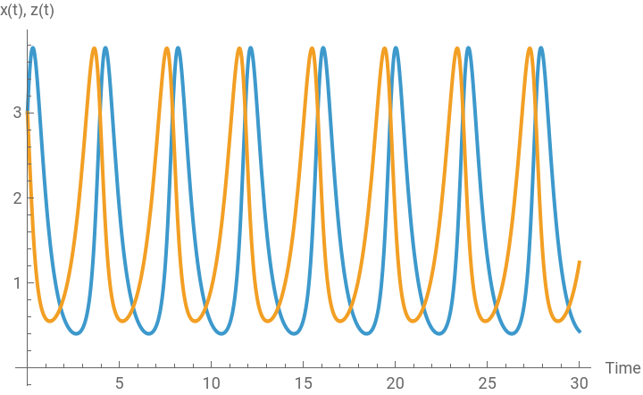
If we assign some arbitrary values to each parameter and set initial values, we can generate the following simulation:
In[]:=
ClearAll[a,c,α,β,γ,x,y,z,t,sol];a=2;α=1.2;c=1.5;γ=1;sol=NDSolve[{x'[t]==-ax[t]+αx[t]z[t],z'[t]cz[t]-γx[t]z[t],x[0]3,z[0]3},{x[t],z[t]},{t,0,30}]
Out[]=
x[t]InterpolatingFunction[t],z[t]InterpolatingFunction[t]


As we can see Figures below, there emerges a classic predator-prey relation in between the rent income and profit income over time. As the gross profit for agricultural capitalists increases, agricultural farmers can lease out a greater unit of arable land to these agricultural capitalists who would cultivate and produce more agricultural products. If this happens, the rent will rise as agricultural capitalists compete with one another to lease the limited land. This process, in turn, ultimately lower the agricultural profits as capitalists are required to pay higher rent. As this happens, capital accumulation in the agricultural sector slows down, so does the rent income with a certain time lag. In this nonlinear dynamical relation between the two income variables, the profit for agricultural capitalists plays a role as a prey, while the rent for the owner of land a predator.
We can visualize this nonlinear dynamic relation in the following two ways: In the first plot, both rent and profit income appear on the vertical axis while the time variable on the horizontal axis. This plot shows how the two income variables behave over time. One variable traces the trajectory of the other.
In the second plot, we put the same rent and profit income variable on both vertical and horizontal axis, thereby showing their interdependent growth trajectory. If one variable (i.e., profit income) grows, the other variable (i.e., rent income) also grows. But as soon as rent income grows in tandem, it generates a negative feedback on the growth of profit income. Ultimately, their interdependent growth trajectory exhibits an orbit circle, having one non-zero steady state value a center.
In[]:=
Plot[Evaluate[{x[t],z[t]}/.sol],{t,0,30},PlotLegends{"rent","profit"},AxesLabel{"Time","x(t), z(t)"}]
Out[]=


We can also draw a phase diagram in which forces in the vector field defined by the very differential equations in the model are visualized. The following Figure shows how we can see the solution curve for the interacting two variables inside this phase diagram.
As in this diagram, the original model can have many complex features. It may have multiple ‘sources’ (points of divergence) as well as ‘sinks’ (points of attraction). We can also observe the possibility of a ‘saddle point’ equilibrium along the values of x = 0 and z = 0. But at least on the positive domain for both x and z variables, we have an orbit circle. Which one of these possibilities will become pronounced depends on the initial value and parameters.
In comparison, we can also draw a 3D phase portrait by assigning some arbitrary parameter values to the original system of three differential equations. Suppose, for example, a=2, α=1.2, b=1.5, β = 1.3, c=1.5, γ=1 and δ = 1.4.
As this 3D plot shows, there is a clearly discernable predator-prey relationship in the domain between rent and profit income. As soon as we introduce a third, inverse wage-profit dynamics, this predator-prey relation turns into a more complex chaotic motion.
An interactive visualization of the solution curves
An interactive visualization of the solution curves
Let us also run another simulation by assigning a range of values for some crucial parameters and creating an interactive chart. For example, let a = 2, b = 1.5, and c = 1.5. Using ParametricNDSolve function in Mathematica, we can generate solution paths of x(t), y(t), and z(t), which are all dependent on the remaining parameters, α, β, γ, δ.
This chaotic interaction among the three variables captured in this phase portrait is similar to either the Lorenz equations (Lorenz 1963) or Chemostat models (Herbert, Elsworth, and Telling 1956). It is also similar to a food chain model of three interacting species (McLaren and Peterson 1991). This line of reasoning provides us with one useful venue for extending Ricardo’s business cycle model. Even though Ricardo himself did not use any mathematical formulation in his exposition of the long-run dynamics of capital accumulation, his high-level inductive reasoning seems to warrant this kind of phase portrait analysis.
Conclusion
Conclusion
In this note, we have sought to replicate David Ricardo’s ‘income-distribution-led business cycle model’ in his Principles. Ricardo’s analysis of the dynamic interaction among the three social class incomes - wages, profits, and ground rent - constitutes one important system model that are quite similar to the Lorenz equation and chemostat model of complexity.
Reference
Reference
◼
Brian E. McLaren and Rolf O. Peterson, “Wolves, Moose, and Tree Rings on Isle Royale,” Science, 266 (1994), pp.1555-58 (https://www.science.org/doi/10.1126/science.266.5190.1555).
◼
Denis Herbert, R. Elsworth, and R.C. Telling, “The Continuous Culture of Bacteria, a
Theoretical and Experimental Study,” Microbiology, Vol. 14, No. 3 (1956), pp.601–622 (https://www.microbiologyresearch.org/content/journal/micro/10.1099/00221287-14-3-601).
Theoretical and Experimental Study,” Microbiology, Vol. 14, No. 3 (1956), pp.601–622 (https://www.microbiologyresearch.org/content/journal/micro/10.1099/00221287-14-3-601).
◼
Edward N Lorenz, “Deterministic Nonperiodic Flow,” Journal of the Atmospheric Sciences, Vol.
20, No.2 (1963 ), pp.130-141 (https://eapsweb.mit.edu/about/history/publications/lorenz)
20, No.2 (1963 ), pp.130-141 (https://eapsweb.mit.edu/about/history/publications/lorenz)
◼
Ricardo, David. 1996 [1821]. Principles of Political Economy and Taxation, Amherst, New York : Prometheus Books.
◼
Shin, Hee-Young. 2022. “A computational approach to Ricardo’s and Marx’s business cycle models” (https://papers.ssrn.com/sol3/papers.cfm?abstract_id=4187298 )
CITE THIS NOTEBOOK
CITE THIS NOTEBOOK
Introduction to dynamic economic models: Ricardo's rent-profit-wage income dynamics & business cycle
by Hee-Young Shin
Wolfram Community, STAFF PICKS, January 4, 2026
https://community.wolfram.com/groups/-/m/t/3600553
by Hee-Young Shin
Wolfram Community, STAFF PICKS, January 4, 2026
https://community.wolfram.com/groups/-/m/t/3600553