Traditional register machines follow deterministic, linear paths with predictable behavior. In this project, we investigate multi-way register machines, which allow multiple possible transitions at each instruction step, producing a branching computation tree. To study their behavior, we develop two types of rule visualizations and construct graphs that showcase all reachable states up to a specified depth. A probabilistic plot further illustrates how instruction and register values evolve on average across all branches at each depth. I also implemented basic arithmetic operations, such as addition, subtraction, multiplication, division, scalar, and power, using multi-way register machines, allowing one to construct arbitrary polynomial equations. Finally, I modeled recursive processes such as the Fibonacci sequence and the Collatz conjecture using this framework.
Traditional register machines follow deterministic, linear paths with predictable behavior. In this project, we investigate multi-way register machines, which allow multiple possible transitions at each instruction step, producing a branching computation tree. To study their behavior, we develop two types of rule visualizations and construct graphs that showcase all reachable states up to a specified depth. A probabilistic plot further illustrates how instruction and register values evolve on average across all branches at each depth. I also implemented basic arithmetic operations, such as addition, subtraction, multiplication, division, scalar, and power, using multi-way register machines, allowing one to construct arbitrary polynomial equations. Finally, I modeled recursive processes such as the Fibonacci sequence and the Collatz conjecture using this framework.
Introduction to Multi-Way Register Machines
Introduction to Multi-Way Register Machines
A register machine is a simple computational model that manipulates a finite number of registers holding non-negative integers, through a sequence of deterministic instructions. Each instruction specifies which register to operate on and whether to increment or decrement its value. In an increment instruction, the machine moves on to the next instruction. However, for a decrement instruction, there are two possible outcomes; if the machine is successfully able to decrement the register specified, then you move to some arbitrary instruction; otherwise, if the register has a value of 0 and cannot decrement any further, then that step is a “fail” and the machine moves on to the next instruction. Register machines are deterministic by nature; there is only one instruction to move to in a given state. Even in a decrement instruction, which might seem like it has two possible instructions to move to, the next move is determined whether it is possible to decrement the given register. The flow of execution follows a fixed, linear path, where each instruction leads to exactly one subsequent instruction, making the machine’s behavior fully predictable given an initial state.
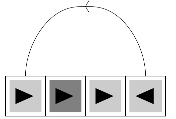
Below is an example of a very simple register machine; the cycle is evident, and one can easily predict the current state given the number of iterations the machine performs.Here, we have 3 increment instructions followed by a decrement instruction. The second instruction modifies the second register, and the other instructions modifies the first register; we can determine this based on the color of the instruction. If the decrement instruction is a success, then we move back to the first instruction. If it is a fail, we can say for simplicity that the machine comes to a halt. It is fairly obvious that this machine will never halt from the fourth instruction failing.
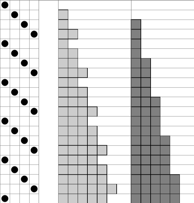
These deterministic register machines are trivial in the sense that you can easily calculate or predict the current state, which we define as the current instruction the machine is reading and the list of values of each register. Below is a table that displays the state at every iteration of the machine, for the first 20 iterations:The instruction index follows a cycle of four and the two registers also follow a very trivial pattern. However, in a multi-way register machine, it has the potential to have more than one option for where to move to. This creates multiple branches that the machine can follow, and over time, will result in a complex graph of possible states.
Multi-Way Register Machine Input Format
Multi-Way Register Machine Input Format
Now that we have multiple options for where to move to on a single instruction, it’s not practical to assume that increment instructions and failed decrement instructions automatically move to the instruction to the right. When creating an machine, we will explicitly mention all possible instructions one can move to. We can describe the components of each instruction to create the rules for the machine. For each instruction, we can either have three or four components; the register to modify, whether to increment or decrement the register (denoted by 0 for increase and 1 for decrease), a list of instructions to move to upon success, and an optional list of instructions to move to upon failure, only present for decrement instructions. Note that the second element, which indicates increment or decrement, can be determined based on the number of elements; 3 elements is an increment instruction, and 4 elements for a decrement one. In this regard, storing this value in the list is redundant. We can even describe single-way Register Machines in this manner; the one above can be characterized as:
In[]:=
SingleWayRM={{1,0,{2}},{2,0,{3}},{1,0,{4}},{1,1,{1},{}}};
The first list corresponds to the first instruction; we have a register with type 1 (shaded light gray) that increments, and it has a directed edge to the second instruction upon a success. The second and third instructions are defined with a similar format. For the fourth instruction is a decrement light gray one; a success would move the counter to the first instruction, and a failure would halt the machine because the fourth element is a empty list.
MRMRulePlot
MRMRulePlot
For demonstration purposes, let’s set the machine to be:
In[]:=
testInstructions={{1,0,{2,3}},{2,1,{1},{3,4}},{2,0,{5}},{1,1,{3,5},{1,5}},{2,1,{1,2},{}}};
Following our input format as outlined earlier, we will create a visualization of the instructions that we give to the machine, defined as MRMRulePlot. First, instead of processing a list based on the attributes of each instruction, we will convert our instructions input into a list whose elements represent each directed edge. The optimal form to achieve this is {instruction index, register index, register to move to, increment/decrement, success/fail edge}. We can create helper functions that takes in an instruction from our instructions input and outputs all the edges that this instruction creates. For simplicity purposes, we will create one specifically for creating success edges and one for creating fail edges.
splitInstructions takes in an instruction and outputs a list of success edges starting at that instruction. splitInstructions2 takes in an instruction and outputs a list of fail edges starting at that instruction. The input idx is used when these functions are called in a MapIndex function, and it represents the current index of the inputted instruction.
In[]:=
splitInstructions[instr_,idx_]:=Table[{First[idx],instr[[1]],instr[[3,i]],instr[[2]],0},{i,Length[instr[[3]]]}]splitInstructions2[instr_,idx_]:=If[Length[instr]==4,Table[{First[idx],instr[[1]],instr[[4,i]],instr[[2]],1},{i,Length[instr[[4]]]}]]
Now we need to iterate through all instructions and merge all the outputted lists. We use the MapIndexed function to do so, which stores each element as well as its index. The latter is necessary to retrieve the instruction index.
We perform MapIndexed with functions splitInstructions and splitInstructions2 iterating across testInstructions. To prevent a double nested list, we flatten it one level.
Flatten[MapIndexed[splitInstructions,testInstructions],1]Flatten[MapIndexed[splitInstructions2,testInstructions],1]
Out[]=
{{1,1,2,0,0},{1,1,3,0,0},{2,2,1,1,0},{3,2,5,0,0},{4,1,3,1,0},{4,1,5,1,0},{5,2,1,1,0},{5,2,2,1,0}}
Out[]=
{Null,{2,2,3,1,1},{2,2,4,1,1},Null,{4,1,1,1,1},{4,1,5,1,1}}
We now want to combine these lists together for MRMRulePlot to use. Note that the outputs could potentially have Null values (as seen here in the second output) caused by instructions not having any success/fail edges. So we ensure that we remove all Null values from our final list.
Combine the two lists from above using Join and use Select to only take the non-Null elements.
Select[Join[Flatten[MapIndexed[splitInstructions,testInstructions],1],Flatten[MapIndexed[splitInstructions2,testInstructions],1]],#=!=Null&]
Out[]=
{{1,1,2,0,0},{1,1,3,0,0},{2,2,1,1,0},{3,2,5,0,0},{4,1,3,1,0},{4,1,5,1,0},{5,2,1,1,0},{5,2,2,1,0},{2,2,3,1,1},{2,2,4,1,1},{4,1,1,1,1},{4,1,5,1,1}}
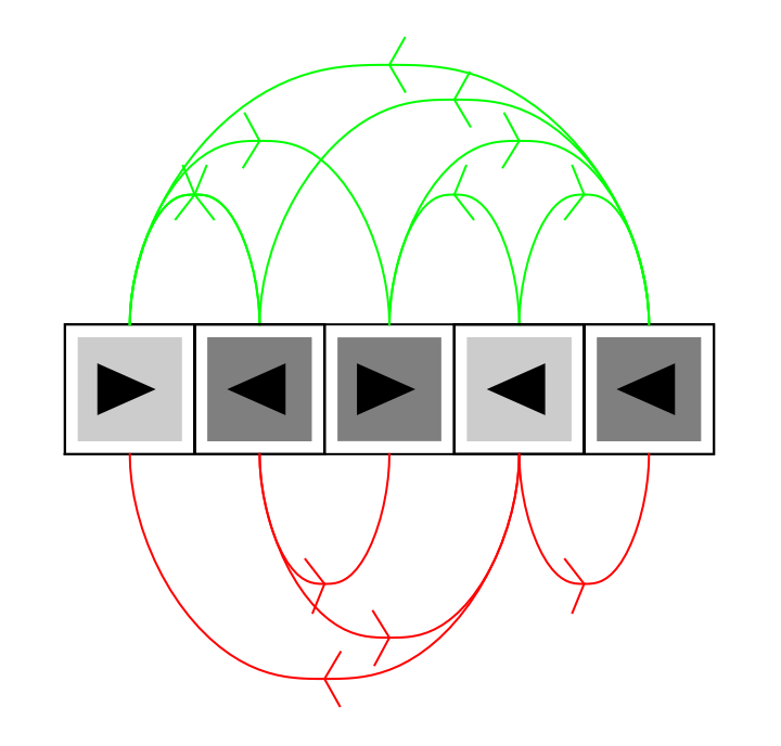
We use this to create the directed edges between instructions; they are created using Arrow and Arrowheads, and success edges will be drawn in green from the top and fail edges drawn in red from the bottom. Additionally, instructions will be denoted as a box with a colored square (indicating the register number) and a direction (indicating whether to increment or decrement the register). The machine itself are the all the instructions in order lined up against each other.
We have to create multiple graphics to entirely visually simulate the machine. First, we create arrowheads for the edges using two lines in an arrow shape. Next, we draw curved arrows from one instruction box to another. It uses a B-spline to make the transitions visually appealing and easier to track. Depending on the increment/decrement status, should be above or below the line of instructions. gfun takes in the register number and total number of registers and creates a color for the register. The first register is a brighter gray, and succeeding registers have a darker and darker shade of color. Finally, we create a triangle and flip it according to whether the current instruction is an increment or decrement. Together, this forms the graphics of MRMRulePlot.
MRMRulePlot creates a visual representation of the instructions and their attributes, as well as how pairs of instructions are connected. The Translate function shifts each instruction and corresponding edges to the right according to the instruction index.
In[]:=
MRMRulePlot[prog_,nreg_Integer:2,opts___]:=Graphics[{Arrowheads[{{-0.02,.5,Graphics[{Line[{{{0,0},{1,Sqrt[3]}},{{0,0},{1,-Sqrt[3]}}}]}]}}],With[{gfun=Interpolation[{{1,.8},{nreg,.5}},InterpolationOrder->1]},MapIndexed[{Translate[{GrayLevel[gfun[#1[[2]]]],Rectangle[{0.1,0.1},{0.9,0.9}],Black,Rotate[Triangle[{{0.7,0.7},{0.25,0.5},{0.7,0.3}}],If[#1[[4]]==0,π,0]],EdgeForm[Black],Opacity[0],Rectangle[{0,0}]},{First[#1],0}],If[Last[#1]==0,Green,Red],Arrow[With[{x1=First[#1]+.5,x2=#1[[3]]+.5,yMax=(Max[1,Sqrt[Abs[First[#1]-#1[[3]]]]]+1-Last[#1])*(1-2*Last[#1])},BSplineCurve[{{x1,1-Last[#1]},{x1,yMax},{(x1+x2)/2,yMax},{x2,yMax},{x2,1-Last[#1]}},SplineWeights->{1,0.5,1,0.5,1}]]]}&,Select[Join[Flatten[MapIndexed[splitInstructions,prog],1],Flatten[MapIndexed[splitInstructions2,prog],1]],#=!=Null&]]]},Sequence[PlotRangePadding->{0.5},{opts}]];
Now we can visualize any instructions input in the form of instructions and directed edges. For example, here is the MRMRulePlot for testInstructions:
MRMRulePlot[testInstructions]
Out[]=
MRMCircPlot
MRMCircPlot
A RulePlot function for a single-way Register Machine like the one in the introduction is practical because there aren’t that many edges. However, in a multi-way machine, especially since we aren’t implying edges between adjacent instructions anymore, the number of edges drastically increase in multi-way Register Machines. This makes the edges of RulePlot a little harder to discern the more edges added. Thus, I feel like the list of instructions in a circle would be more practical in this case.
The MRMCircPlot function outputs a visual representation of a multi-way register machine by placing each instruction node evenly around a circle (unlike MRMRulePlot) and drawing arrows to indicate the possible transitions between them. Each node corresponds to a numbered instruction, and is labeled with its index for clarity. Similar to MRMRulePlot, we use green arrows to denote a success edge and red arrows for a fail edge. For each instruction, a directional triangle is drawn inside the node to indicate whether the operation increments (left-pointing triangle) or decrements (right-pointing triangle) the register. This circular layout makes it easy to visually trace all potential transitions in the program logic, identify loops, and understand the structural flow of the machine in a compact format. The function first computes the position of each instruction on the circle, then constructs arrows using a helper function (findArrows) that handles the directional logic, colors, and placement of each edge. Finally, it renders the full diagram with all nodes and transitions using Graphics.
In[]:=
MRMCircPlot[prog_,nreg_Integer:2]:=Module[{n=Length[prog],positions,arrows,radius=3,nodeRadius=0.25,arrowInset=0.3,gfun},gfun=Interpolation[{{1,.8},{nreg,.5}},InterpolationOrder->1];positions=Association@Table[i->radius{Cos[2Pi(i-1)/n],Sin[2Pi(i-1)/n]},{i,n}];arrows=First@Nest[findArrows[prog,positions,arrowInset],{{},1},n];Graphics[{arrows,Table[With[{pos=positions[i],regType=prog[[i,1]],dirSym=If[prog[[i,2]]==0,Polygon[{{0.08,0},{-0.08,0.08},{-0.08,-0.08}}],Polygon[{{-0.08,0},{0.08,0.08},{0.08,-0.08}}]]},{EdgeForm[Black],GrayLevel[gfun[regType]],Disk[pos,nodeRadius],Black,Translate[dirSym,pos],Text[Style[ToString[i],Bold,12],pos,{0,-1.5}]}],{i,n}]},PlotRange->All,ImageSize->500]]findArrows[prog_,positions_,arrowInset_][{arrows_,i_}]:=Module[{t=prog[[i]],succPCs,failPCs,p1,p2,dir,newArrows},If[t[[2]]==0,succPCs=t[[3]];newArrows=Join[arrows,Table[p1=positions[i];p2=positions[pc];dir=Normalize[p2-p1];{Green,Arrow[{p1+arrowInset*dir,p2-arrowInset*dir}]},{pc,succPCs}]],succPCs=t[[3]];failPCs=t[[4]];newArrows=Join[arrows,Table[p1=positions[i];p2=positions[pc];dir=Normalize[p2-p1];{Green,Arrow[{p1+arrowInset*dir,p2-arrowInset*dir}]},{pc,succPCs}],Table[p1=positions[i];p2=positions[pc];dir=Normalize[p2-p1];{Red,Arrow[{p1+arrowInset*dir,p2-arrowInset*dir}]},{pc,failPCs}]];];{newArrows,i+1}]
We can compare MRMRulePlot and MRMCircPlot on testInstructions, to compare how easily one can discern its edges.
Personally, MRMCircPlot is much more interpretable than MRMRulePlot in this situation. Each has its pros and cons; one should use MRMRulePlot for simpler machines that have fewer edges and more instructions. One should use MRMCircPlot for machines with more edges and fewer instructions, since a large array of instructions can make it confusing.
Complexity of a Multi-Way Register Machine
Complexity of a Multi-Way Register Machine
On the topic of the number of instructions compared to the edges, we can create a function to quantify the complexity of a given machine. We can define complexity to be how often the machine creates new branches on average. A machine with a greater number of edges relative to its vertices has a higher complexity, and vice versa. We will create a simplistic function that may not accurately model the complexity across all machines; however it would be a very good estimate. For every instruction in the program, it calculates the average number of outgoing success and (if a decrement instruction) failure transitions.
For decrement instructions, the function ensures that the failure edge count is at least 1, even if the failure list is empty. This avoids underestimating complexity in cases where a failure is unreachable in the machine; for example, the machine SingleWayRM has an empty fail list because it cannot fail. Without this correction, some instructions might appear simpler than they actually are.
After computing this average for every instruction, it then takes the geometric mean of all those values to get a single complexity score for the entire machine. The geometric mean is used instead of the arithmetic mean because it better represents the multiplicative or exponential growth of branching paths, making it a more sensitive measure for machines with highly variable structure. The final result is a real number that reflects how often the machine creates new branches.
Let’s test the complexity of a single-way Register Machine.
A complexity of one represents no increase in the number of paths. This makes sense, because the machine follows only one path. On the other hand, a machine like testInstructions should have a higher complexity.
This means on average each path splits into 1.55 new paths upon every iteration. Some limitations of this function representing a machine’s complexity include ones that have a halting instruction, which are instructions that have no outgoing edge. This would be guaranteed to bring the complexity of the machine to 0, as you are taking the geometric mean of a list with 0 in it. This hides the potential complexity of the machine due to a single instruction.
The most complex machine would have all of its instructions form a fully connected graph. The complexity of the graph would be the number of instructions minus 1.
Simple Multi-Way Register Machine
Simple Multi-Way Register Machine
Even the simplest multi-way register machines can have chaotic behavior. Let’s take the single-way register machine from above and add an edge from the second instruction to the fourth instruction. So our instructions to the machine are now the following:
Essentially, the machine now has the option to skip the third instruction and can do so whenever it pleases. Since the number of possible branches doubles every 4 instructions, it’s apparent that even one additional edge will exponentially increase the number of paths as the depth increases, where depth means the number of execution steps. Since we now have a function that computes the complexity of a machine, let’s use it.
One can reach a particular state through multiple paths, which leads to a cyclic graph rather than a tree. This motivated me to create a representation of a machine through its potential states through a graph, where we define a state to be {instruction counter, {list of register values}}. The nodes of the graph represent the possible states, and we include directed edges between nodes that can reach each other in one iteration.
MRMEvolveGraph
MRMEvolveGraph
The goal of function MRMEvolveGraph is to create a graph that includes all states {instruction counter, {list of register values}} and the directed edges that connect them. We have several helper functions that we use to conduct this process.
The MRMStep function simulates a single instruction execution in a multi-way register machine. It takes a program and a state represented by an instruction pointer and a list of register values. If the current instruction is out of bounds, it halts immediately. Otherwise, it checks whether the instruction is an increment or decrement. For increment instructions (length 3), it increments the appropriate register and returns a list of all possible next states. For decrement instructions (length 4), it checks whether the register can be decremented; if so, it decrements it and returns the next states based on the success list. If the register is zero, the machine cannot decrement it and instead returns the unchanged registers with the instruction pointing to the failure list.
The function MRMStep simulates a single instruction step and returns all possible next states.
The handleTransition function ensures the uniqueness of transitions in the graph. Given a source state ID and a new state to transition into, it checks whether that transition has already been recorded. If not, it adds a new edge between the states and updates the edge tracking structure. This function returns the new state, along with the updated edge set and list of edges.
The function handleTransition adds a transition between two states if it hasn’t been recorded yet.
The expandState function processes one state from the queue. It first determines all possible next states using MRMStep, and then for each of these, it calls handleTransition to safely track any new edges or states. It returns a list of newly discovered states to explore, and the updated edge tracking structures.
The function expandState applies MRMStep to a state and processes all resulting transitions.
The processQueueLevel function processes all states at the current depth level in a breadth-first search. For each state in the queue, it expands it into its child states using expandState, accumulates all resulting new states into a new queue, and merges all edge updates. It returns the new queue and updated edge information for the next layer of the BFS.
The function processQueueLevel processes all states at the current BFS level and returns the next queue.
These helper functions are used to create the function MRMEvolveGraph. It initializes all required structures to keep track of visited states, assign unique state IDs, and store the transitions as edges. It defines a helper function getID that assigns a unique integer to each unique machine state. It begins the BFS from the initial state and repeatedly calls processQueueLevel until it reaches the specified depth or runs out of states. At the end, it constructs and returns a Graph object with all discovered states and transitions.
The function MRMEvolveGraph evolves the register machine state graph up to a max depth using BFS.
This function is especially useful as a good visualization of the cycles and intersecting paths that the machine has as we increase the depth. Observing the evolution of the graph as the depth changes is particularly insightful.
We can create a slider to model the evolution of MRMEvolveGraph on simpleMRM.
Interpretation of MRMEvolveGraph
Interpretation of MRMEvolveGraph
We created a graph depicting all possible states that the machine can be in within a certain depth and how to get there. These graphs can get complicated as the depth increases. As an example, let’s consider the machine simpleMRM, which only has one additional edge from a single-way Register Machine, and its MRMEvolveGraph with depth 50.
For simplicity purposes, let’s analyze the graph with a smaller maximum depth.
We initially start at {1, {0, 0}}, which is the default starting position; our counter is currently at 1, and the values of both registers are 0. To move from the first instruction, we have to increment the first register by 1. We can only move to the second instruction, so that’s the only possible state. From there, we increment the second register by 1 and now we can either move to the third or fourth instruction. This creates two outgoing edges and splits the graph into two paths. Each path is a valid set of instructions that the machine can perform. MRMEvolveGraph encompasses all possible paths that the machine can follow.
MRMProbPlot
MRMProbPlot
The aim of this model is to visualize how the machine behaves in general, across all branches, at each depth. We do this by creating a list of columns of boxes at each depth. The first element represents the possible locations and their probabilities that the instruction index can go to. Each of the remaining elements represents a register, and each box n (for n=1, 2, 3...) represents the probability that the register has a value of n or greater. We represent probability by setting the opacity of each object; black means there is a 100 percent chance of the object appearing in this location, and white means a 0 percent chance. We begin by writing this function by creating a couple of helper functions, the first being MRMStatesAtDepth.
MRMStatesAtDepth is used to simulate every possible state of the machine at a certain depth. It takes three inputs: the program (prog), an initial state (init), and a target depth (targetDepth). This function uses NestList to iteratively apply a function that advances the machine one step: that function maps MRMStep over the current list of states and flattens the resulting lists into a single new list. In other words, at depth 0, it starts with just the initial state; at depth 1, it applies one step to produce all states reachable in a single transition; at depth 2, it applies another step to each of those, and so on, until it has done exactly targetDepth iterations. Finally, by extracting the last element of the NestList result, it returns the complete, flattened list of all states the machine can occupy after exactly that many steps.
Create the function MRMStatesAtDepth as outlined above.
We can test this function out on simpleMRM.
These are all possible states that the machine can reach in exactly 6 moves.
Now we look at another helper function, MRMProbList, which generates the nested list of probabilities of possible counter positions and register values, as outlined earlier.
First, we define the function and immediately collect all reachable states at the given depth using our helper function MRMStatesAtDepth. If there are no states (in the event that the machine has halted), we return an empty list. Then, we look at the distribution of the instruction counters. We extract the instruction indices from each state, find the maximum index, and compute the frequency of each index. Dividing by the total count gives the probability distribution over instruction counters, as desired. Now we look at each register. For each register, we build a list of probabilities over time: for thresholds n=1 to maxVal, we compute the fraction of states whose register value is at least k. This yields one probability list per register, and we can append these values into a list. Append the register probability lists to the instructions probability list.
The function MRMProbList is a helper function to MRMProbPlot that generates a list of lists for the probability of a counter existing at every instruction and values of every register up to a certain depth.
Let’s test this on simpleMRM:
The probability of the counter being at the first and third instructions is 25% each, and a 50% chance of being at the fourth instruction. Additionally, from the next two lists we can infer that the first register has a 75% chance of having a value of 2, and the second register has a value of 2 regardless of what path we took.
Now we can finally create the function MRMProbPlot. We have the list of possibilities from MRMProbList and we can run this function for every depth. However instead of lists, we will interpret the data as a table of boxes with opacities representing the probabilities.
First we will create a module and define the variables needed. We call MRMProbList repeatedly for every depth from 0 to maxDepth, storing the results in a list called summaries. This forms the raw data we’ll use to create the entire probabilistic plot. We then find the widest instruction probability list so we can layout the horizontal axis appropriately. Next, we draw disks for the instruction index at each depth. Each disk’s horizontal position corresponds to the instruction index i. Vertical position is the depth (negated to make the timeline go downward). The opacity of each black disk corresponds to how likely it is for the machine to be at that instruction index at that particular step.
Then we build the actual probability plot for each register. At each depth, and for each possible token value k, we draw a rectangle. The opacity of the black square corresponds to the probability that the register has a value of at least k. These are plotted from left to right (increasing value) and stacked vertically (increasing depth). Finally, we use GraphicsRow to place the instruction plot (made of disks) and the register plots (made of squares) side by side. The Spacings option adds a little padding between columns.
The function MRMProbPlot averages out the potential states of the machine at each depth and displays it neatly in multiple tables.
Once again, we can test this function on simpleMRM.
As seen in MRMEvolveGraph, the initial state and first iteration of this machine is deterministic; Thus the first two rows have fully black (probability of 100%) disks and squares. At depth 2, however, we can go to the third or fourth instruction, with equal probability. This is why two disks are displayed in the first table at the third column, each with opacity 0.50. Beyond this depth, the values in the registers aren’t necessarily determined; paths may have different values of registers at the same depth. However, it is apparent in this graphic that the second register increases much faster than the first register.
Complete Register Machines
Complete Register Machines
Now that we have created the functions necessary, we can explore some interesting cases of multi-way Register Machines. We can start with a compete multi-way Register Machine; one that every instruction is connected by every other instruction. The machine would look like the following, for three instructions:
Let’s take a look at its MRMRulePlot.
We have three increment instructions for the same register, each with edges to the other two instructions. We can analyze the structure of the graph of possible states that this machine produces.
This follows a very trivial pattern, especially for a multi-way Register Machine. There are usually three nodes in every column, and there are two ways for one to move to the next column. At every increase of depth by 1, it appears that the number of paths doubles. To check this fact, we can observe the complexity of the machine:
This is expected as this machine is a complete graph with 3 nodes. The MRMProbPlot is also something very expected.
As depth increases, the probabilities of the counters appearing on instructions approach each other to be equal. The counter has a higher chance of appearing on the first instruction on the first few iterations, however it is only due to the counter initially starting there.
We can easily assume that similar things happen for a complete graph with more instructions; for n instructions the complexity would be n-1 and number of paths would scale by (n-1) on every iteration of the machine.
Halting Register Machines
Halting Register Machines
A halting Register Machine has an instruction with an empty success/fail list. When the machine reaches this instruction, there is a chance that the path simply ends. This would decrease the complexity of the graph compared to one that doesn’t halt. The lessened complexity could potentially appear in functions MRMEvolveGraph and MRMProbPlot, though. Let’s define a machine as:
The complexity of this graph is:
This is a halting Register Machine because the sixth instruction has no outgoing success edges. Since you can only get to the sixth instruction from the fifth instruction, which increments the second register, it is impossible to fail this instruction and we are guaranteed to halt once we reach this.
Let’s compare this machine to one that doesn’t halt at the sixth instruction; we modify the outgoing edges so that the complexity of the two machines are identical.
We expect the complexity to be equal between machines.
Let’s analyze the MRMEvolveGraph of the halting machine.
We can tell where the paths halt; when we have states that branch out from the “main” graph and then end, we know that the machine has reached instruction 6 and cannot proceed any further. Let’s test our non-halting machine to see if there is any discrepancy.
We can clearly see that that non-halting machine is much more complex than the halting one. More paths are generated because they now continue beyond the sixth instruction. Now, let’s test MRMProbPlot to see if the halting instruction is notable.
We see that the first register value doesn’t diverge in general, while the second register does. The second register diverges because there is only one decrement register of that kind, and when you reach it the machine halts. For the counter, it seems more likely to be on the third or fourth instructions than any others. Now apply MRMProbPlot on the non-halting Machine.
Now both registers diverge, however the second one diverges much slower than the halting Machine. Although both machines have identical complexity, there are discernible differences between them. This also shows the limitations of the function complexity, since the halting machine has less complexity in practice.
Modeling Polynomials Using Register Machines
Modeling Polynomials Using Register Machines
We will start with modeling the function y=kx (where k is some constant nonnegative integer), and we can do so with two registers. We start with the state {1, {x, 0}}, and we want to explore a certain branch of a certain machine that has the state {_, {0, kx}}, where the instruction counter doesn’t really matter. We do this using a decrement instruction of the first register followed by k increment instructions of the second register. All instructions, upon success, will move onto the next instruction (and cycling around if necessary). When the decrement instruction fails, the machine halts. Due to these particular rules, we get that for every decrement of the first register by 1, the second register increments by k. This is exactly what we need to multiply numbers by a scalar. We can generate the machine itself using Table.
The function scalar takes in a nonnegative integer k and outputs a list of one decrement instruction of register 1 followed by k increment instructions of register 2. An optional variable next tells to which instructions to go to once the decrement instruction fails. We also have a shift variable if you need to shift over where the edges go; such as when we use this function in the middle of a machine.
Similarly, we can create the function divide, which takes an integer and divides it by some constant positive integer k. If the integer doesn’t properly get divided, then we take the ceiling. This function operates similarly to scalar, except that we have k decrement instructions and 1 increment instruction. When we run out of value from the first register, we immediately halt or get sent to next.
The function divide takes in a positive integer k and divides any integers by k, taking the ceiling if necessary.
To model the function z=xy (where k is some constant positive integer), we are going to need 4 registers. We want to start with the state {1, {y, x, 0, 0}}\b and end with state {_, {0, x, 0, xy}}. First, we will decrement the first register by 1 and move to the second instruction. We repeatedly decrease the second register by 1 and increase the third and fourth registers by 1, until we deplete the second register. Then, we shift the value of the third register to the second register. After one iteration of this, we will be at state {_, {y-1, x, 0, x}}. Repeating this once again, and we will be at state {_, {y-2, x, 0, 2x}}. We can continue repeating this until the first register hits zero, and by then we will be at state {_, {0, x, 0, xy}} as desired. Once again, we can create a function to create the machine to multiply two numbers together.
The function multiply creates the registers, instructions, and edges needed to multiply two numbers together. An optional variable next tells to which instructions to go to once this process is over. We also have a shift variable if you need to shift over where the edges go; such as when we use this function in the middle of a machine.
The power function provides the framework to raise a number to a power.
Finally, we create an addition and subtraction function. These are the simplest ones; we start from state {1, {x, y}} and end at state {1, {0, x+y}}. For addition, we simply shift the values of the first register to the second.
The function add sums two integers together.
For subtraction, we decrease both registers until one of them hits zero. If y is greater than x, then we will start at state {1, {x, y}} and end at {_, {0, y-x}}.
The function subtract takes the difference of two integers. The output is stored in the greater integer’s register.
We create the machine using power, scalar, and add. Each one should use the proper k value (if needed), should have the proper shift and list of registers, moving to the next function accordingly.
Create a list of MRMStatesAtDepth at every depth until a large number; only select lists that aren’t empty (if a list is empty then the machine has halted by now) and return the last element, which should be the desired state.
Modeling the Collatz Sequence Using Multi-Way Register Machines
Modeling the Collatz Sequence Using Multi-Way Register Machines
Now that we can create polynomial functions using multi-way Register Machine, we can simulate the Collatz Sequence. We start at a certain state {1, {n, 0}} and apply the rules of the Collatz Sequence; if n is odd, we multiply by 3 and add 1, and if n is even then we divide by 2. So, one of the instructions should have two outgoing edges depending on the parity of n. For 3n+1, we use scalar with a k value of 3 and add 1. For n/2, we use divide with a k value of 2.
Let’s check the complexity of this machine.
The only additional branch here to instruction 8, where when we fail, we go to instruction 4 if the first register has an odd value and instruction 6 otherwise. We create a custom function, inspired by MRMStatesAtDepth, that chooses the correct path to take when the machine reaches the eighth instruction.
The function collatzSimulate takes the multi-way Register Machine that computes the Collatz Sequence. It begins with an initial state, which should be of the form (for initial integer N) {8, {0, N}} and evolves the machine for a fixed number of steps (maxDepth). For each iteration up to maxDepth, it loops over the current states and generates the next possible states. However, unlike MRMStatesAtDepth, there is a special case when the machine hits instruction 8. If the first register is 0, it checks the parity of the second register. If the second register is odd, it moves to instruction 4; otherwise, it moves to instruction 6. For all other instructions, it behaves normally; either incrementing or decrementing registers and moving to the next instructions based on success or failure conditions. The simulation collects all the next states and adds them to the running list allStates. In the end, it returns the particular branch that defines the Collatz Sequence.
The function collatzSimulate simulates one specific branch of collatzInstructions, by handling a special case at instruction 8 to branch based on whether the second register is odd or even.
Let’s test this function using a starting value of 5.
The very last state is {8, {0, 1}}, which represents when the machine should technically “halt,” since the Collatz Sequence is conjectured to transform every integer to 1.
The function collatzSequence extracts the Collatz Sequence generated by the function above. It takes in an integer N, which represents the starting value for the Collatz process. The function first calls collatzSimulate with collatzInstructions defined above, and an initial state where instruction 8 is the starting point and the second register holds the value N. It runs the simulation for 20,000 steps to ensure we actually reach 1. After collecting all possible states, it filters the list to include only those that occur when the counter is on instruction 8 and the first register is 0, indicating that an iteration is complete. It then extracts the value of the second register from these states to form the sequence. Finally, it returns the list truncated at the first occurrence of 1, which is when the Collatz Sequence ends.
The function collatzSequence extracts the actual Collatz Sequence from the path generated by collatzSimulate by filtering states that meet the final-instruction condition and collecting register values until 1 is reached.
We test this with initial value 101.
Checking, we see that the rules of the Collatz Sequence are indeed followed here. We triple and add 1 to odd numbers, and halve even numbers.
Modeling the Fibonacci Sequence Using Multi-Way Register Machines
Modeling the Fibonacci Sequence Using Multi-Way Register Machines
We can create the Fibonacci Sequence as well using this logic. We will use four register machines, starting with state {1, {1, 1, 0, 0}}. The first two Fibonacci numbers are in the first and second registers. We start by moving the value of the second register into the third and fourth registers. We then take the sum of the first and third registers and store it in the third register. Finally, we move the value of the third register to the second and the fourth to the first. Iteratively repeating this process yields pairs of the Fibonacci sequence. Let’s now create the machine to do so.
We can output the Fibonacci numbers using a similar method as polynomialCreater, where we use MRMStatesAtDepth to find all the states for the machine up until a depth. We know when we are done with one iteration of the Fibonacci Sequence when the counter is at the first instruction, and the third and fourth registers are set to 0. So we can select only those states to look at. The Fibonacci numbers themselves appear in the first register of these selected states.
We iterate through the machine 2000 times and only select the states which have finished one cycle of the over process. With those states, we output the first register value.
This list is indeed the first 10 Fibonacci numbers, so we can use this function to generate any Fibonacci number.
Conclusion
Conclusion
Through this project, I explored the power and flexibility of multi-way register machines as a computational model. I developed a range of visual tools, including RulePlot, CircPlot, complexity, ProbPlot, and EvolveGraph, to analyze the structure and behavior of these machines. With these tools in place, I designed register machine programs that perform basic arithmetic operations like addition, subtraction, multiplication, and division, as well as scalar and power functions. These building blocks allowed me to represent general polynomial functions with integer coefficients entirely with multi-way Register Machine. I extended this work to model recursive processes such as the Fibonacci sequence and the Collatz conjecture. Altogether, this project not only deepened my understanding of discrete computation but also showed how surprisingly expressive simple register-based systems can be.
Future Directions
Future Directions
Moving forward, one compelling area of exploration is the study of register growth behavior over time using probabilistic tools. By using MRMProbPlot, we can visualize how values in each register evolve as the machine progresses through multiple steps, which could help us identify machines with linear or chaotic growth rates. Similarly, we can analyze whether certain instructions are used disproportionately compared to others through the use of MRMProbPlot, providing insight into the internal structure of a machine’s execution. These kinds of usage patterns might reflect deeper organizational principles or point to instruction sets that are naturally more efficient.
Another valuable direction is the analysis of edge-case Register Machines. For example, machines composed solely of success transitions, or ones that lack failure paths entirely, may exhibit fundamentally different behaviors than typical machines. Likewise, self-looping instructions, where the next instruction can points to itself, can create stagnation or infinite loops that are important to observe. We can also study convergence and divergence in the evolution graphs generated by MRMEvolveGraph.
Finally, in the standard multi-way Register Machine used here, each instruction can only increment or decrement a register by exactly 1. There’s no built-in way to change a register by more than 1 in a single step. Allowing instructions to increment/decrement registers by more than one or even zero could yield more interesting results, such as more cycles in MRMEvolveGraph.
References
References
Wolfram Physics Project. (2021, February). Multiway Turing machines. Wolfram Physics Bulletin. https://bulletins.wolframphysics.org/2021/02/multiway-turing-machines/
Wolfram, S. (2002). A new kind of science (p. 100). Wolfram Media. https://www.wolframscience.com/nks/p100--register-machines/
Wolfram, S. (2002). A new kind of science (p. 100). Wolfram Media. https://www.wolframscience.com/nks/p100--register-machines/
Acknowledgements
Acknowledgements
I would like to thank my mentor, Dan McDonald (we published this on our birthday!), for helping me throughout this project; digging through literature, debugging frustrating code, or suggesting new directions to explore. He also believed in my project enough to advocate for it directly with Stephen Wolfram, which made this whole experience possible. Without him, I wouldn’t have had the chance to work on something this interesting. I’d also like to thank all the Wolfram staff, including the directors, mentors, and TAs, who put together the 2025 Wolfram Summer Research Program and gave me the tools and space to take this project as far as I could, making the experience more enjoyable in the process.
CITE THIS NOTEBOOK
CITE THIS NOTEBOOK
State evolution in multiWay register machines featuring applications to recursive functions
by Pratham Mukewar
Wolfram Community, STAFF PICKS, July 10, 2025
https://community.wolfram.com/groups/-/m/t/3499350
by Pratham Mukewar
Wolfram Community, STAFF PICKS, July 10, 2025
https://community.wolfram.com/groups/-/m/t/3499350