Solution of a Steady-State Heat Conduction Problem using the Galerkin Method
Authors: Housam Binous and Ahmed Bellagi
Solution of a Steady-State Heat Conduction Problem using the Galerkin Method
Authors: Housam Binous and Ahmed Bellagi
Authors: Housam Binous and Ahmed Bellagi
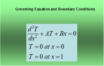
Exact Solution
In[]:=
sol=DSolve[{D[T[x],{x,2}]+AT[x]+Bx0,T[0]0,T[1]0},T[x],x]
Out[]=
T[x]
-Bx+BCsc[
A
]Sin[A
x]A
One -Term Trial Solution
Approximate Solution using the Galerkin Method
Approximate Solution using the Galerkin Method
In[]:=
T2a[x_]:=c1[x]
ϕ
1
In[]:=
ϕ
1
In[]:=
R1=Integrate[[x](D[T2a[x],{x,2}]+AT2a[x]+Bx),{x,0,1}]
ϕ
1
Out[]=
B
12
c1
3
Ac1
30
In[]:=
sys={R1==0}
Out[]=
-+0
B
12
c1
3
Ac1
30
In[]:=
sol1=Solve[sys,{c1}]
Out[]=
c1-
5B
2(-10+A)
In[]:=
%/.A1/.B1
Out[]=
c1
5
18
Two-Term Trial Solution
Approximate Solution using the Galerkin Method
Approximate Solution using the Galerkin Method
In[]:=
T2[x_]:=c1[x]+c2[x]
ϕ
1
ϕ
2
In[]:=
ϕ
1
In[]:=
ϕ
2
In[]:=
R1=Integrate[[x](D[T2[x],{x,2}]+AT2[x]+Bx),{x,0,1}]
ϕ
1
Out[]=
B
12
c1
3
Ac1
30
c2
6
Ac2
60
In[]:=
R2=Integrate[[x](D[T2[x],{x,2}]+AT2[x]+Bx),{x,0,1}]
ϕ
2
Out[]=
B
20
c1
6
Ac1
60
2c2
15
Ac2
105
In[]:=
sys={R1==0,R2==0}
Out[]=
-+-+0,-+-+0
B
12
c1
3
Ac1
30
c2
6
Ac2
60
B
20
c1
6
Ac1
60
2c2
15
Ac2
105
In[]:=
sol2=Solve[sys,{c1,c2}]
Out[]=
c1,c2-
(70+A)B
420-52A+
2
A
7B
-42+A
In[]:=
%/.A1/.B1
Out[]=
c1,c2
71
369
7
41
Comparing Exact and Approximate Solutions
In[]:=
xd=Table[x,{x,0.0,1.0,0.05}]
Out[]=
{0.,0.05,0.1,0.15,0.2,0.25,0.3,0.35,0.4,0.45,0.5,0.55,0.6,0.65,0.7,0.75,0.8,0.85,0.9,0.95,1.}
In[]:=
tbl1=Table[First[T[x]/.sol],{x,0.0,1.0,0.05}]/.A1/.B1
Out[]=
{0.,0.009395,0.0186415,0.0275915,0.0360977,0.0440137,0.0511948,0.0574981,0.0627829,0.0669109,0.069747,0.0711589,0.0710184,0.0692006,0.0655851,0.0600562,0.0525025,0.042818,0.0309019,0.016659,0.}
In[]:=
tbl2a=Table[First[T2a[x]/.sol1],{x,0.0,1.0,0.05}]/.A1/.B1
Out[]=
{0.,0.0131944,0.025,0.0354167,0.0444444,0.0520833,0.0583333,0.0631944,0.0666667,0.06875,0.0694444,0.06875,0.0666667,0.0631944,0.0583333,0.0520833,0.0444444,0.0354167,0.025,0.0131944,0.}
In[]:=
tbl3a=Quiet[100(tbl2a-tbl1)/tbl2a]
Out[]=
{Indeterminate,28.7958,25.4338,22.0945,18.7803,15.4938,12.2375,9.01403,5.82572,2.67504,-0.435628,-3.50392,-6.52753,-9.50419,-12.4317,-15.3078,-18.1306,-20.8978,-23.6075,-26.2577,Indeterminate}
In[]:=
tbl2b=Table[First[T2[x]/.sol2],{x,0.0,1.0,0.05}]/.A1/.B1
Out[]=
{0.,0.00954505,0.0188537,0.0277978,0.0362493,0.0440803,0.0511626,0.0573682,0.0625691,0.0666372,0.0694444,0.0708628,0.0707642,0.0690207,0.0655041,0.0600864,0.0526396,0.0430356,0.0311463,0.0168438,0.}
In[]:=
tbl3b=Quiet[100(tbl2b-tbl1)/tbl2b]
Out[]=
{Indeterminate,1.57206,1.12506,0.741855,0.418386,0.151157,-0.0628694,-0.226347,-0.341617,-0.410757,-0.435628,-0.417906,-0.359114,-0.260645,-0.123781,0.0502873,0.260448,0.505657,0.784926,1.09731,Indeterminate}
In[]:=
Join[{{x,Exact,Approx,Perc.Error,Exact,Approx,Perc.Error}},Transpose[{xd,tbl1,tbl2a,tbl3a,tbl1,tbl2b,tbl3b}]]//MatrixForm
Out[]//MatrixForm=
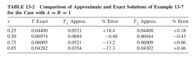
x | Exact | Approx | Perc.Error | Exact | Approx | Perc.Error |
0. | 0. | 0. | Indeterminate | 0. | 0. | Indeterminate |
0.05 | 0.009395 | 0.0131944 | 28.7958 | 0.009395 | 0.00954505 | 1.57206 |
0.1 | 0.0186415 | 0.025 | 25.4338 | 0.0186415 | 0.0188537 | 1.12506 |
0.15 | 0.0275915 | 0.0354167 | 22.0945 | 0.0275915 | 0.0277978 | 0.741855 |
0.2 | 0.0360977 | 0.0444444 | 18.7803 | 0.0360977 | 0.0362493 | 0.418386 |
0.25 | 0.0440137 | 0.0520833 | 15.4938 | 0.0440137 | 0.0440803 | 0.151157 |
0.3 | 0.0511948 | 0.0583333 | 12.2375 | 0.0511948 | 0.0511626 | -0.0628694 |
0.35 | 0.0574981 | 0.0631944 | 9.01403 | 0.0574981 | 0.0573682 | -0.226347 |
0.4 | 0.0627829 | 0.0666667 | 5.82572 | 0.0627829 | 0.0625691 | -0.341617 |
0.45 | 0.0669109 | 0.06875 | 2.67504 | 0.0669109 | 0.0666372 | -0.410757 |
0.5 | 0.069747 | 0.0694444 | -0.435628 | 0.069747 | 0.0694444 | -0.435628 |
0.55 | 0.0711589 | 0.06875 | -3.50392 | 0.0711589 | 0.0708628 | -0.417906 |
0.6 | 0.0710184 | 0.0666667 | -6.52753 | 0.0710184 | 0.0707642 | -0.359114 |
0.65 | 0.0692006 | 0.0631944 | -9.50419 | 0.0692006 | 0.0690207 | -0.260645 |
0.7 | 0.0655851 | 0.0583333 | -12.4317 | 0.0655851 | 0.0655041 | -0.123781 |
0.75 | 0.0600562 | 0.0520833 | -15.3078 | 0.0600562 | 0.0600864 | 0.0502873 |
0.8 | 0.0525025 | 0.0444444 | -18.1306 | 0.0525025 | 0.0526396 | 0.260448 |
0.85 | 0.042818 | 0.0354167 | -20.8978 | 0.042818 | 0.0430356 | 0.505657 |
0.9 | 0.0309019 | 0.025 | -23.6075 | 0.0309019 | 0.0311463 | 0.784926 |
0.95 | 0.016659 | 0.0131944 | -26.2577 | 0.016659 | 0.0168438 | 1.09731 |
1. | 0. | 0. | Indeterminate | 0. | 0. | Indeterminate |
In[]:=
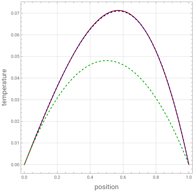
plt1=Plot[T[x]/.sol/.A1/.B1,{x,0,1},PlotStyleDarker@Red,Frame->True,GridLines->Automatic,FrameLabel->{Style["position",14],Style["temperature",14]},AspectRatio->1,ImageSize->400{1,1}];
In[]:=
plt2=Plot[T2[x]/.sol2/.A1/.B1,{x,0,1},PlotStyle{Dashed,Darker@Blue},Frame->True,GridLines->Automatic,FrameLabel->{Style["position",14],Style["temperature",14]},AspectRatio->1,ImageSize->400{1,1}];
In[]:=
plt2a=Plot[T2a[x]/.sol2/.A1/.B1,{x,0,1},PlotStyle{Dashed,Darker@Green},Frame->True,GridLines->Automatic,FrameLabel->{Style["position",14],Style["temperature",14]},AspectRatio->1,ImageSize->400{1,1}];
comparison of exact solution and the two approximate solutions
In[]:=
Show[plt1,plt2,plt2a]
Out[]=