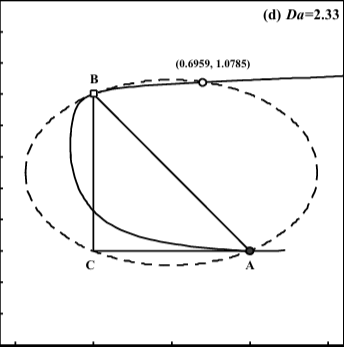
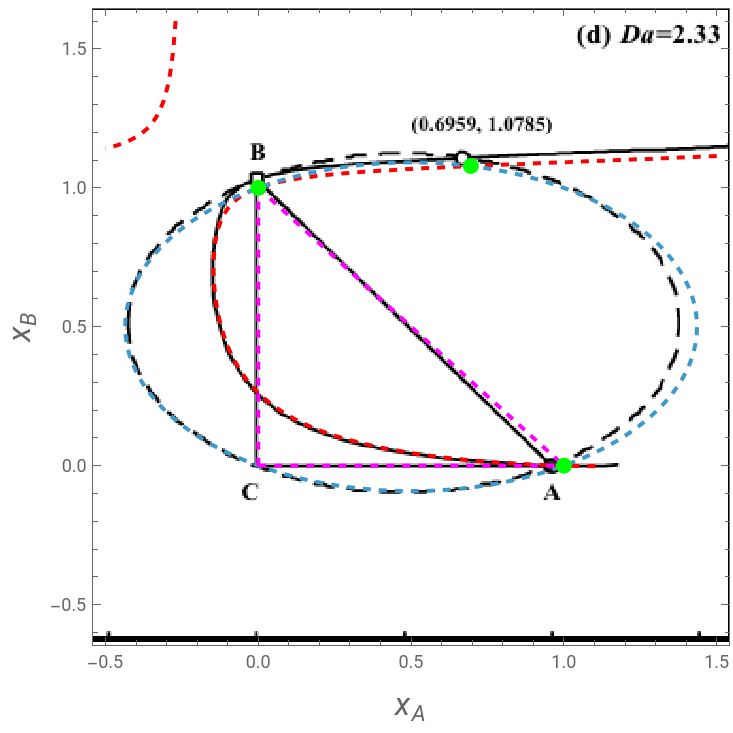
We shows how one can easily reproduce the Figures 5.14 and 5.15 (pages 113-114) of Ref. 1 using ContourPlot command.
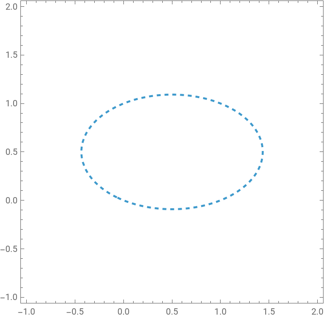
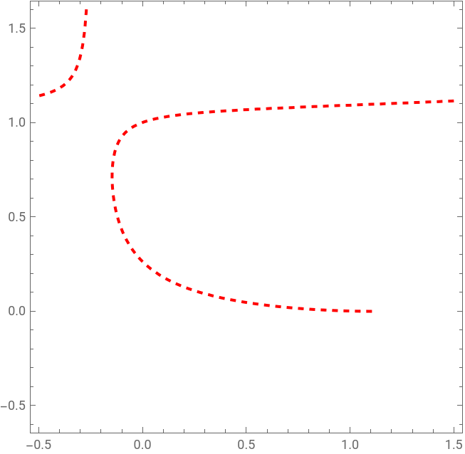
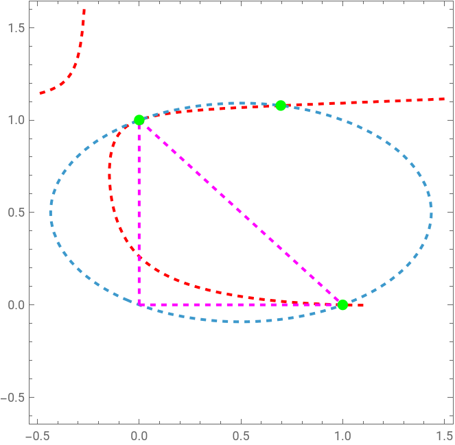
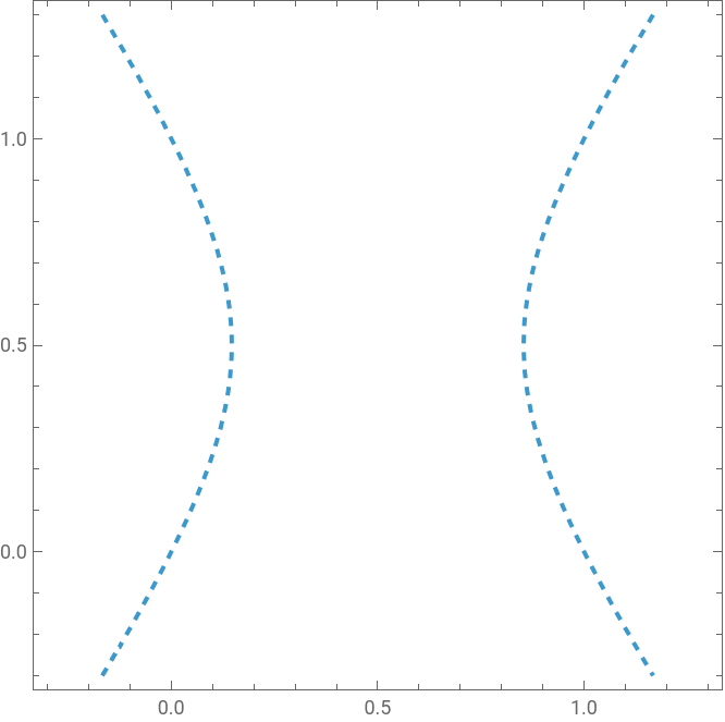
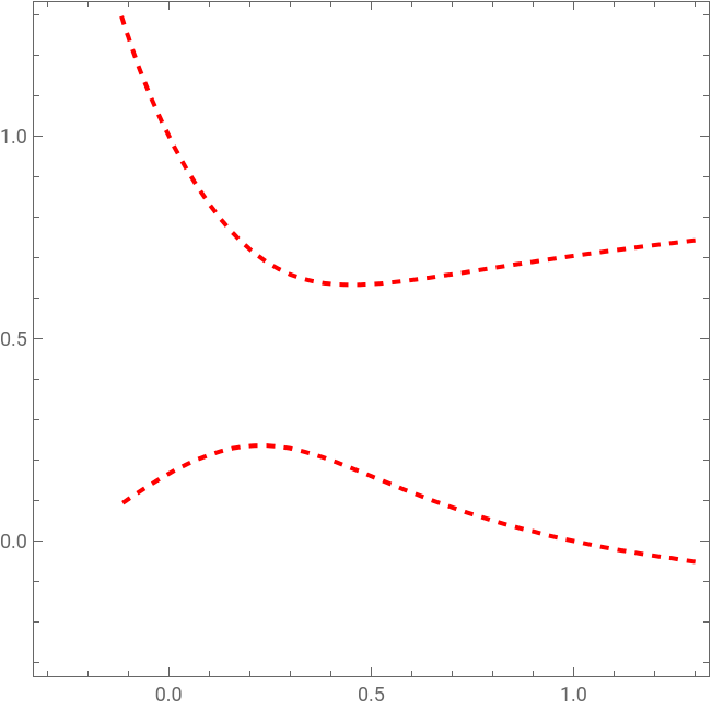
Applying singular point analysis to reactive distillation, one determines the attainable bottom composition of an infinitely high counter-current RD column operated at infinite reflux. This attainable compositions are the stable node, which is calculated from the intersection of the kinetic curve (shown in red) and singular point curve (shown in blue).
Applying singular point analysis to reactive distillation, one determines the attainable bottom composition of an infinitely high counter-current RD column operated at infinite reflux. This attainable compositions are the stable node, which is calculated from the intersection of the kinetic curve (shown in red) and singular point curve (shown in blue).
Case a: =0.2and=3.0
α
13
α
23
Singular point curve
In[]:=
y3=1-y1-y2;x3=1-x1-x2;
In[]:=
y1=x1/(x1+x2+x3);y2=x2/(x1+x2+x3);
α
21
α
31
α
12
α
32
In[]:=
eq=(x1+x3)(1+y3)-(y1+y3)(1+x3);
In[]:=
α
21
α
12
α
31
α
32
In[]:=
plt1=ContourPlot[eq0,{x1,-1,2},{x2,-1,2},RegionFunctionFunction[{x1,x2},Evaluate[Abs[eq]<1.0]],ContourStyle->{Dashed,Thick}]
Out[]=
In[]:=
eq2=-(y2-x2)+(-1+x2)Da(x1x2-x3/K);
Kinetic curve for Damköhler number Da=2.33
In[]:=
K=5;Da=2.33;
In[]:=
plt2=ContourPlot[eq20,{x1,-0.5,1.5},{x2,-0.6,1.6},RegionFunctionFunction[{x1,x2},Evaluate[Abs[eq]<1.0]],ContourStyle{Dashed,Thick,Red}]
Out[]=
In[]:=
sol=FindRoot[{eq0,eq20},{x1,0.8},{x2,1.7}]
Out[]=
{x10.695511,x21.07854}
In[]:=
A=Show[plt2,plt1,Graphics[{{Dashed,Thick,RGBColor[1,0,1],Line[{{0,0},{0,1}}]},{Dashed,Thick,RGBColor[1,0,1],Line[{{0,0},{1,0}}]},{Dashed,Thick,RGBColor[1,0,1],Line[{{0,1},{1,0}}]},{RGBColor[0,1,0],PointSize[0.025],Point[{x1/.sol,x2/.sol}]},{Dashed,Thick,RGBColor[0,1,0],PointSize[0.025],Point[{1,0}]},{RGBColor[0,1,0],PointSize[0.025],Point[{0,1}]}}]]
Out[]=
In[]:=
img=
;
In[]:=
Show[A,ImageSize->400{1,1},Prolog->{Raster[ImageData[img,DataReversed->True],{Scaled[{-0.02,0.005}],Scaled[{1,1.}]}]},FrameLabel->{Style["",16,Italic],Style["",16,Italic]}]
x
A
x
B
Out[]=
Case b: =5.0and=3.0
α
13
α
23
In[]:=
α
21
α
12
α
31
α
32
Singular point curve
In[]:=
plt3=ContourPlot[eq0,{x1,-0.3,1.3},{x2,-0.3,1.3},RegionFunctionFunction[{x1,x2},Evaluate[Abs[eq]<1.0]],ContourStyle->{Dashed,Thick}]
Out[]=
Kinetic curve for Damköhler number Da=1.5
In[]:=
K=5;Da=1.5;
In[]:=
eq2=-(y2-x2)+(-1+x2)Da(x1x2-x3/K);
In[]:=
plt4=ContourPlot[eq20,{x1,-0.3,1.3},{x2,-0.3,1.3},RegionFunctionFunction[{x1,x2},Evaluate[Abs[eq]<1]],ContourStyle{Dashed,Thick,Red}]
Out[]=
In[]:=
sol1=FindRoot[{eq0,eq20},{x1,0.8},{x2,0.7}]
Out[]=
{x10.87732,x20.686388}
In[]:=
sol2=FindRoot[{eq0,eq20},{x1,0.08},{x2,0.3}]
Out[]=
{x10.0912648,x20.20995}
In[]:=
A=Show[plt4,plt3,Graphics[{{Dashed,Thick,RGBColor[1,0,1],Line[{{0,0},{0,1}}]},{Dashed,Thick,RGBColor[1,0,1],Line[{{0,0},{1,0}}]},{Dashed,Thick,RGBColor[1,0,1],Line[{{0,1},{1,0}}]},{RGBColor[0,1,0],PointSize[0.025],Point[{x1/.sol1,x2/.sol1}]},{RGBColor[0,1,0],PointSize[0.025],Point[{x1/.sol2,x2/.sol2}]},{RGBColor[0,1,0],PointSize[0.025],Point[{1,0}]},{RGBColor[0,1,0],PointSize[0.025],Point[{0,1}]}}]]
References
References
◼
[1] K. Sundmacher & Z. Qi, Importance of Reaction Kinetics for Catalytic Distillation, Reactive Distillation, Status and Future Directions, Edited by Kai Sundmacher & Achim Kienle, Wiley VCH, 2002.
CITE THIS NOTEBOOK
CITE THIS NOTEBOOK
Singular point analysis in reactive distillation
by Housam Binous and Ahmed Bellagi
Wolfram Community, STAFF PICKS, September 8, 2025
https://community.wolfram.com/groups/-/m/t/3541802
by Housam Binous and Ahmed Bellagi
Wolfram Community, STAFF PICKS, September 8, 2025
https://community.wolfram.com/groups/-/m/t/3541802