In this project, we investigate how different axiom systems affect the possible theorems that are provable and which are decidable. We explore how the different combinations of axioms lead to different patterns of decidability, and deduce the complex patterns that arise when combining axioms.
Introduction
Introduction
The field of mathematics is built upon assumptions on how the mathematical world ought to work. Every field of math, from group theory to boolean algebra has assumptions that are central to the field’s existence. Finding the smallest possible axiom system for these fields is therefore important: it would reduce the number of assumptions needed for proofs, making them cleaner, as well as set a basis for further investigation of the minimal axiom system. In essence, mathematicians want to find the smallest logically sound foundations that are equivalent to logical theories.
Knuth-Bendix completion algorithm
Knuth-Bendix completion algorithm
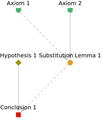
The Knuth-Bendix completion algorithm is an algorithm that transforms a set of identities into a logically equivalent confluent term rewriting system. A reduction system s is confluent if, for all w,x,y such that w eventually reduces to x and y, there exists a z such that x and y both eventually reduce to z. The algorithm can be used to find if other identities hold, and is used as the primary algorithm behind the FindEquationalProof function. FindEquationalProof finds if there is a path to the theorems from the axioms provided, and it returns a ProofObject that represents the proof in its entirety.
Proves the transitive property of equality
In[]:=
proof=FindEquationalProof[a==c,{a==b,b==c}]
Out[]=
ProofObject


Shows a graph that represents the proof
In[]:=
GraphPlot[proof["ProofGraph"],ImageSize->Small]
Out[]=
Analysis of single-axiom systems
Analysis of single-axiom systems
An axiom is defined as a statement that is assumed in a field of math, and from which other statements, known as theorems, are proven. For the purposes of this project, axioms will be constructed by equivocating two different expressions, both of which contain a maximum of two variables, as well as a binary operator that relates the two. As we want to try our best to minimize assumptions, it is necessary to also introduce a grouping mechanism that shows order of operations, which parentheses will be used for. Due to the relative simplicity of the axiom system we assume, it is possible to generate a list of all possible axioms and theorems up to a certain level of complexity.
A list of axioms and theorems
axioms=;theorems=;
Notice how the axioms and theorems use completely different variables. This is because the axioms do not relate constants, but they relate variables, which means that the axioms can act as pattern replacement rules. This is most obvious in the proof to prove a theorem like p=(p·p)·q from a=a·b.
Outputs the proof graph for p=(p·p)·q with a=a·b as an axiom
In[]:=
GraphPlot[FindEquationalProof[p==(p·p)·q,ForAll[{a,b},a==a·b],TimeConstraint->0.3]["ProofGraph"],ImageSize->Small]
Out[]=
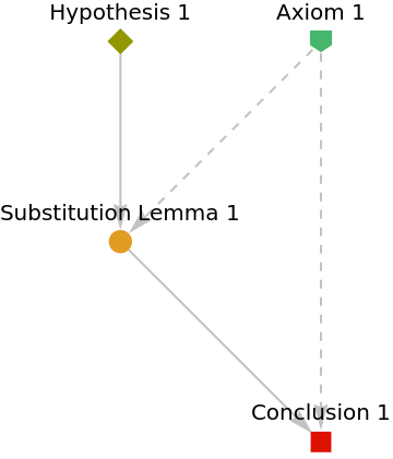
From the hypothesis to substitution lemma 1, if one uses the rule a_·b_a_, one can find that p·p=p, which completes the first step. The rest of the proof is trivial. This entire process is automated using the FindEquationalProof function, which means that we can find the theorems that this axiom proves as well.
Finds the theorems provable from a=a·b; theorems that are provable are in dark blue
In[]:=
ResourceFunction["https://www.wolframcloud.com/obj/wolframphysics/PlotTheoremArray"][{{a==a·b},theorems}->{ParallelTable[If[ResourceFunction["HeadQ"][FindEquationalProof[i,ForAll[{a,b},a==a·b],TimeConstraint->0.3],ProofObject],3,0],{i,theorems}]}]
Out[]=

This allows us to analyze different axiom systems easily with our theorems. We can thus analyze every single axiom we have right now.
Finds all theorems that are provable using the axioms we have defined
In[]:=
ResourceFunction["https://www.wolframcloud.com/obj/wolframphysics/PlotTheoremArray"][{axioms,theorems}->ParallelTable[If[ResourceFunction["HeadQ"][FindEquationalProof[j,ForAll[{a,b},i],TimeConstraint->0.3],ProofObject],3,0],{i,axioms},{j,theorems}]]
Out[]=
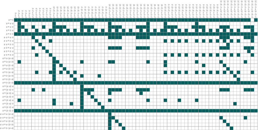
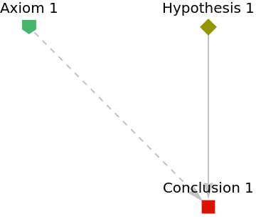
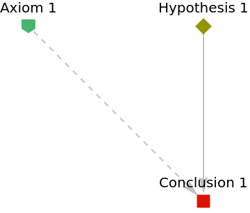
Note some interesting patterns in the grid. In essence, there is a pattern of the theorems on the diagonal trivially proving themselves, and another pattern of some axioms proving every theorem. For example, the axiom a=b proves every result. This is also extremely easy to see intuitively, as it is clear that every single statement follows the pattern a_=b_.
Proof graphs from a=b to two arbitrarily chosen theorems (note how they look exactly the same)
In[]:=
{GraphPlot[FindEquationalProof[RandomChoice[theorems],ForAll[{a,b},a==b],TimeConstraint->0.3]["ProofGraph"],ImageSize->Small],GraphPlot[FindEquationalProof[RandomChoice[theorems],ForAll[{a,b},a==b],TimeConstraint->0.3]["ProofGraph"],ImageSize->Small]}
Out[]=
,
Adding an axiom
Adding an axiom
Very few mathematical disciplines assume only a single axiom, however. Thus, the next step is to analyze multi-axiom systems. We will start with analysis of two-axiom systems and trying to find if merging two axioms follows a pattern.
Function that takes in two axioms in the form of a list and analyzes them against the list of all theorems
In[]:=
merge[merged_List]:=[{{merged[[1]],merged[[2]],{merged[[1]],merged[[2]]}},theorems}->ParallelTable[If[ResourceFunction["HeadQ"][FindEquationalProof[i,j,TimeConstraint->0.3],ProofObject],3,0],{j,{ForAll[{a,b},merged[[1]]],ForAll[{a,b},merged[[2]]],{ForAll[{a,b},merged[[1]]],ForAll[{a,b},merged[[2]]]}}},{i,theorems}]]
This output follows the pattern of “proving everything”, just like the single axiom a=b
In[]:=
merge[{a==a·b,a==b·a}]
Out[]=

Some axioms are completely unnecessary; in this case, the axiom a=a·b proves a=a·a
In[]:=
merge[{a==a·b,a==a·a}]
Out[]=

This system combines in a strange way
In[]:=
merge[{a·b==b·a,a·b==a·a}]
Out[]=

This system is seemingly logically equivalent to the previous system
In[]:=
merge[{a·a==b·b,a·b==a·a}]
Out[]=

Something that could explain the strangeness of the above two systems is the fact that the only theorems they can prove have at least two variables on each side. This is because it is impossible to reduce systems that only relate two variables to a system that only has one variable. It is completely possible that these behave similarly to the axiom system a=b with very specific limitations.
These two axioms combine in a much nicer and more predictable way
In[]:=
merge[{a·a==b·b,a·b==b·a}]
Out[]=

This merge breaks all established patterns
In[]:=
merge[{a·a==b·a,a==a·a}]
Out[]=

Seemingly, it is logically equivalent to the axiom system a=b·a
In[]:=
This merge produces a grid that is not logically equivalent to any axiom we establish
Finding logical equivalence
Finding logical equivalence
The most interesting patterns with axiom merging are when it results in more theorems being proven than the individual theorems that each axiom prove themselves. To investigate these patterns, it is important to identify which merges are predictable and which are not. The predictable patterns are where the axiom system proves a=b and thus proves everything, or when one of the axioms proves another. To help with this, it is necessary to make a few new functions.
Tests if two statements prove each other; returns True if one of them do and False if not
Returns a list of all axioms in our set of axioms that is stronger than the input axiom
Returns a list of all axioms in our set of axioms that is stronger than the input list of axioms
We will be testing axioms on the system a·a=b·a.
All axioms that are not proven from a·a=b·a and do not prove a·a=b·a
Outputs the result grid for all axioms in combination with a·a=b·a, not including obvious cases like when one proves the other
Now, there are a few patterns in this output grid. Obviously, some axioms prove the result p=q, which makes every single axiom true, There are a few others that follow the familiar idea of every single outcome being proven true except for the theorems with only one variable. However, there are also a few other interesting outcomes, which are all notably logically equivalent to each other. For example, the rows for a=a·(a·a), a=a·(b·a), a=b·(b·a) are all logically equivalent. We can analyze this system further with the functions we made previously.
Finds single axioms that are equivalent or stronger than the axiom system {a=a·(a·a), a·a=b·a}
While there are four axioms here that simply prove every single statement true, there are also two axioms that don’t: a=b·a and a=b·(a·a). We can plot them against {a·a=b·a, a=a·(a·a)}, {a·a=b·a, a=a·(b·a)}, {a·a=b·a, a=b·(b·a)} to find out if they’re stronger or logically equivalent.
Compares the two single axioms with the axiom systems
In fact, for the other pairs of logical equivalence, there also exists a single axiom that is logically equivalent.
Shows logical equivalence of a·b=b·(b·b) and three systems
Shows logical equivalence of a=b·a and five systems
We can also do a deep dive into the proof graphs for all these logical equivalences. While there are four similar outputs, that’s because three of them are just stronger versions of the first one.
Graphs that prove the system a=b·a from its logical equivalences
This is a similar story, as all axioms besides the first one is just a stronger version of another axiom.
Graphs that prove the system a·b=b·(b·b)from its logical equivalences
Same story with these plots.
Graphs that prove the system a=b·(a·a) from its logical equivalences
Overall, it seems that many axioms that result in the same axiom at the end arise from various different strengths of one statement. However, there is no clear pattern between the graphs and how a logically equivalent axiom is constructed from two other axioms.
Negation and internal consistency
Negation and internal consistency
The main limitation of this system is that there is no system of negation. This makes it impossible to do analysis on which theorems are explicitly true in a system, and which theorems are explicitly false. Right now, we only know the explicitly true theorems, and there are no false theorems, but rather theorems that are not decidable from the axioms assumed. Thus, we need to have a system of negation to analyze not only which theorems are true, but, more importantly, which theorems are false. Our system of negation will be simple. We will define ¬a=b and ¬b=a. Further, we will define negation to be distributive over the binary operator. For example, ¬(a·b) will be equivalent to ¬a·¬b. This ends up as a system where negating an axiom just means flipping all variables on one side of an equation.
Function that takes in an axiom and returns its negation
The code requires a bit of a workaround. There are no real tools for symbol manipulation, and negation can only be done through the means of string manipulation, so we must convert it to a string and back to an expression. Further, the axioms themselves break if their negation evaluates to be True in Wolfram Language. We can only input symbols into FindEquationalProof, so it is much easier to convert a and b to the temporary variables c and d before converting them back in the FindEquationalProof process by relating c and d to b and a.
Now, we should talk about the concept of an inconsistent axiom system. We say an axiom system α is inconsistent if and only if it proves a statement and its negation. We notate this as α⊢⊥. In mathematics, we want to avoid inconsistent axiom systems due to the principle of explosion: if a contradiction is true, then any statement can be proven, and thus, contradictions should be avoided at all costs. With a negation system, it becomes paramount to analyze which axioms are consistent by themselves, and further, which axioms are consistent with other axioms. Thus, it would be helpful to create a function that does such a thing.
Function that formalizes all axiom systems, which is important as it allows us to analyze axiom systems easier
Function that takes in an axiom system and shows which axioms it proves, and which it negates
The inconsistency of a=b may have been obvious, but now it has been formally shown in our system
Tests the consistency of a=b
The Law of Excluded Middle shows up naturally.
Tests the consistency of a=a·b
The last test is interesting, as you may have noticed it was able to prove every single theorem or its negation. If this pattern continues, then the axiom would be complete, which means that it is able to decide the truth value of every single theorem. While not proven, the completeness of a=a·b in our system can be investigated further. Of course, the negation of that will also be seemingly complete.
Tests the consistency of a=b·a
A very nice result is that the “2-variable a=b” case is also proven to be inconsistent
As well as this case
And this case
This is all a weird quirk of the fact that commutativity itself is inconsistent
Every single system of axioms seems to be either inconsistent or can be represented by a different single axiom. Obviously, if an axiom system is decided true in another axiom system, merging them would simply be the same as the other axiom system. Similarly, if an axiom system is decided false in another axiom system, merging them would simply lead to an inconsistent result.
A note is that we cannot prove that an axiom system is consistent, we can only prove that an axiom system is inconsistent. Gödel’s 2nd Incompleteness Theorem shows that a system cannot prove its own consistency, which means that it is impossible to actually prove with just our analysis.
Attempted proof
Attempted proof
Unifying axiom for boolean algebra
where · is the Sheffer stroke or the NAND operator. There was a lot of interesting casework done, which we will go through later, but this result has actually been proven to be undecidable; Ralph McKenzie has proven the undecidability of the problem back in 1996 by reducing the Tarski Finite Basis Problem, a weaker version of this theorem, to the halting problem. Specifically, the Tarski Finite Basis Problem asks if it is possible to axiomatize a finite algebra with a finite number of equations. A proof for this reduction can be found here. However, there may still be room to prove the result that all algebras that can be axiomatized by a finite number of equations can also be axiomatized by one equation.
The easiest way to prove this result was to prove mutual undecidability, which states that if two axioms, α and β cannot decide each other, then α and β are consistent. This could be used to show a contradiction when we assume a single-axiomatization does not exist. However, this statement does not hold. There exists a counterexample with {a=b·(a·b),a·a=b·a}:
Tests if a=b·(a·b) and a·a=b·a prove each other.
Shows the inconsistency of {a=b·(a·b), a·a=b·a}
Conclusion
Conclusion
This project explores how two statements may react in a mathematical system, and it explores implications about the axiomatization of statements in systems. We explored the dynamics of equational logic with an elementary 2-variable system, and how different statements from that system can interact in ways that may not be wholly obvious. We then came up with a system of negation, and explored the conditions needed for a combination of statements to be inconsistent. In the end, while there was not a substantive result, there are still two different conjectures that require further investigation, including one that may have large implications for the field of universal algebra itself.
Future Directions
Future Directions
◼
Prove or disprove (or find undecidable) the theorem earlier that stated there exists a single-axiomatization for the case of 2 variables and 1 binary operator
◼
Explore systems with more than 2 variables and more than 1 boolean operator, as well as experiment with different forms of negation.
◼
Prove or disprove that if an algebra has a finite-axiomatization, it can be axiomatized by one axiom.
References
References
◼
Sakharov, Alex. “Knuth-Bendix Completion Algorithm.” From MathWorld--A Wolfram Resource, created by Eric W. Weisstein. https://mathworld.wolfram.com/Knuth-BendixCompletionAlgorithm.html.
◼
Rowland, Todd; Sakharov, Alex; and Weisstein, Eric W. “Confluent.” From MathWorld--A Wolfram Resource. https://mathworld.wolfram.com/Confluent.html
◼
Wolfram, S. (2022, March 7). The physicalization of metamathematics and its implications for the foundations of mathematics. Stephen Wolfram Writings. https://writings.stephenwolfram.com/2022/03/the-physicalization-of-metamathematics-and-its-implications-for-the-foundations-of-mathematics/
◼
Wolfram, S. (2002). A new kind of science (pp. 772–821). Wolfram Media.
◼
MCKENZIE, R. (1996). TARSKI’S FINITE BASIS PROBLEM IS UNDECIDABLE. International Journal of Algebra and Computation, 06(01), 49-104.
Acknowledgements
Acknowledgements
I would like to thank my mentor Henry Gustafson for his metamathematical help throughout the project and for advocating this project, as well as to Adam Millar, who helped in my exploration of the system. Additional thanks to the program directors of WSRP, who are Rory Foulger, Eryn Gillam, Megan Davis, as well as all the other mentors, TAs, and staff that made this camp possible. Final thank you to Stephen Wolfram, who helped in proposing the project and who gave resources on background reading before this project.
CITE THIS NOTEBOOK
CITE THIS NOTEBOOK
Minimal assumptions for mathematics
by River Yu
Wolfram Community, STAFF PICKS, July 11, 2025
https://community.wolfram.com/groups/-/m/t/3501676
by River Yu
Wolfram Community, STAFF PICKS, July 11, 2025
https://community.wolfram.com/groups/-/m/t/3501676