RDKit is an open-source cheminformatics toolkit that allows the manipulation and visualization of molecules (through a suitable representation) on the computer. As an example of its widespread usage, it is the workhorse behind Molecule and most of the functionality related to molecular computation built into Mathematica.
A paper by Sereina Riniker and Greg Landrum features the use of a heatmap (called a "similarity map" in that paper) to visualize differences in molecular fingerprints computed by RDKit, based on the summation of weighted Gaussians () centered at the atom positions of the 2D representation of a molecule. The RDKit documentation also shows an example of the use of heatmaps to visualize molecular descriptors (of the kind computed by MoleculeValue) that are computed on a per-atom basis. (This is similar to what MoleculeValuePlot does.) One can also do a heatmap visualization for per-bond properties (see e.g. the Python code here by Christian Feldmann), but I will restrict myself to per-atom heatmaps here.
--
2
x
2
y
In this notebook, I will demonstrate the use of DensityPlot (and later, DensityPlot3D) to show these heatmaps.
To start things off, consider the Molecule for the insecticide thiamethoxam, generated from its SMILES string representation:
mol=MoleculeModify[Molecule["Clc1ncc(s1)CN2/C(=N\\[N+]([O-])=O)N(C)COC2"],"ComputeAtomDiagramCoordinates"]
Out[]=
Molecule


MoleculePlot[mol]
Out[]=
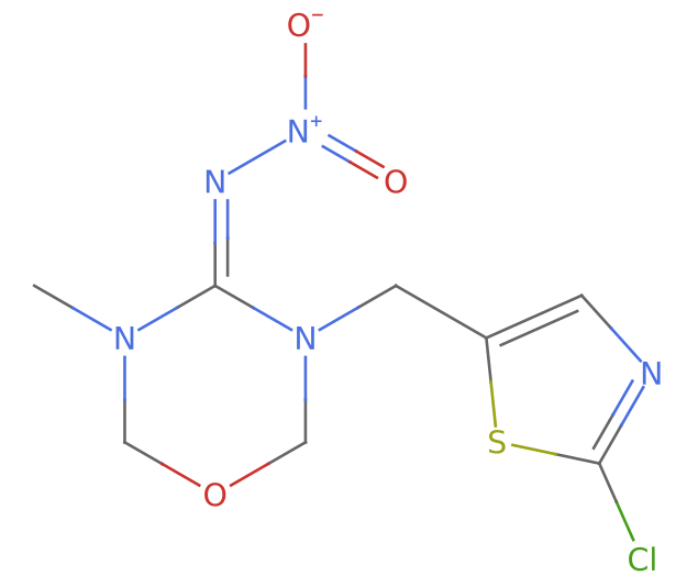
(Note the use of MoleculeModify["ComputeAtomDiagramCoordinates"] to precompute the required atom positions, which will be needed later.)
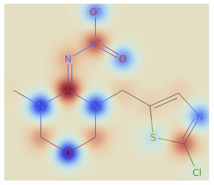
Suppose that we want to visualize the Gasteiger partial charges of the atoms in thiamethoxam. To do that, we first get the coordinates and Gasteiger charges for each atom, using MoleculeValue. (We're mostly interested in the "heavy atoms", or the non-hydrogen atoms, so we will be using the option setting IncludeHydrogensNone frequently in what follows):
coords2d=MoleculeValue[mol,"AtomDiagramCoordinates",IncludeHydrogensNone]
Out[]=
{{2.74163,-2.21361},{2.3349,-1.30007},{2.8349,-0.434041},{2.16577,0.309104},{1.25222,-0.097633},{1.35675,-1.09215},{0.386195,0.402367},{-0.47983,-0.097633},{-1.34586,0.402367},{-1.34586,1.40237},{-0.47983,1.90237},{-0.47983,2.90237},{0.386195,1.40237},{-2.21188,-0.097633},{-3.07791,0.402367},{-2.21188,-1.09763},{-1.34586,-1.59763},{-0.47983,-1.09763}}
gasteiger=MoleculeValue[mol,"GasteigerPartialCharges",IncludeHydrogensNone]
Out[]=
{-0.0505172,0.183343,-0.233179,0.0445398,0.0454623,-0.105734,0.0592376,-0.308888,0.277228,0.101039,0.194106,-0.232597,-0.232597,-0.317195,0.0117906,0.12317,-0.340625,0.12385}
Riniker and Landrum construct the function to be plotted as a weighted sum of Gaussians (see e.g. the Python implementation in RDKit here). In Mathematica, we can do something like the following:
In[]:=
hmfun[x_?NumericQ,y_?NumericQ]:=With[{sc=0.3},Total[MapThread[#2Exp[-SquaredEuclideanDistance[{x,y},#1]/(2sc^2)]&,{coords2d,gasteiger}],Method"CompensatedSummation"]]
We can now look at the heatmap, overlaid with the molecular diagram:
Block{xm,xp,ym,yp},(*computeboundsfortheheatmapfromtheatomcoordinates,plussomepadding*){{xm,xp},{ym,yp}}=MinMax[#,Scaled[0.05]]&/@Transpose[coords2d];ShowDensityPlothmfun[x,y],{x,xm,xp},{y,ym,yp},,MoleculePlot[mol]
Out[]=
Block{xm,xp,ym,yp},{{xm,xp},{ym,yp}}=MinMax[#,Scaled[0.05]]&/@Transpose[coords2d];ShowContourPlothmfun[x,y],{x,xm,xp},{y,ym,yp},,MoleculePlot[mol]
Out[]=
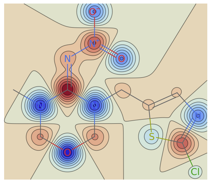
I personally find that the contours do not really add much to the heatmap (and are even a little distracting), so let's stick with using DensityPlot.
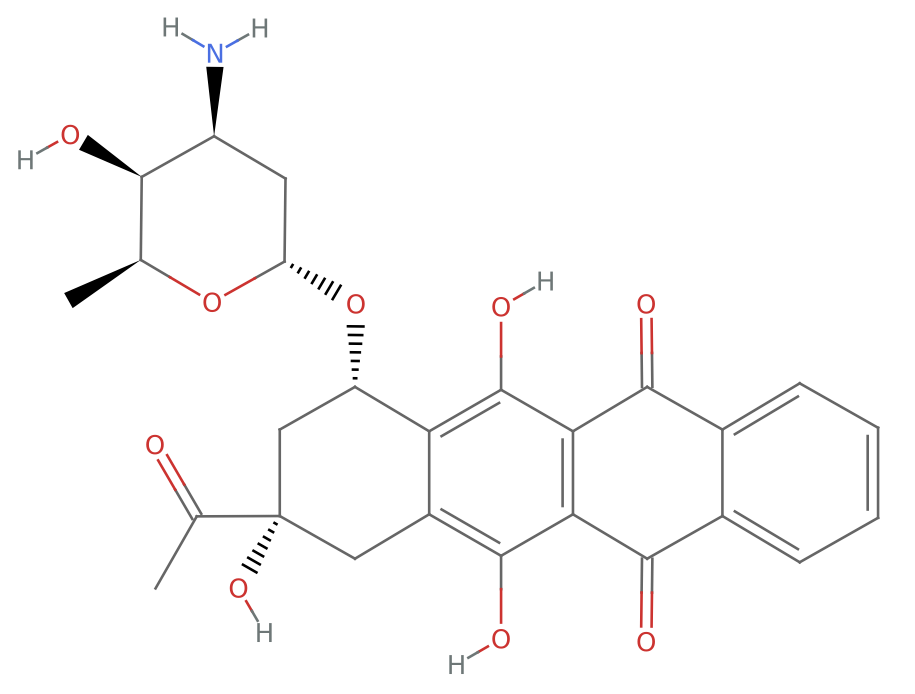
Let's try doing another heatmap, this time using a larger molecule like the antineoplastic antibiotic idarubicin. There is an Entity["Chemical"] corresponding to that molecule, so let's use that:
mol2=Molecule
Out[]=
Molecule

MoleculePlot[mol2]
Out[]=
To change things a bit, let's look at a heatmap visualizing the topological steric effect index for idarubicin's atoms:
coords2da=MoleculeValue[mol2,"AtomDiagramCoordinates",IncludeHydrogensNone]
Out[]=
{{5.9812,0.5043},{4.2493,0.5243},{4.5669,-2.9191},{2.5405,2.5442},{7.7296,0.4697},{7.7296,-3.5303},{3.5603,-1.1909},{9.478,0.5043},{9.478,-3.5649},{4.284,3.5241},{5.9697,-0.4956},{5.0636,-2.0511},{5.0636,-1.0095},{5.9697,-2.565},{6.8636,-1.0303},{6.8636,-2.0303},{5.121,1.0143},{5.1326,2.0142},{4.2724,2.5242},{3.4007,2.0342},{3.3891,1.0343},{7.7296,-0.5303},{4.0636,-2.055},{7.7296,-2.5303},{8.5957,-1.0303},{8.5957,-2.0303},{2.5174,0.5443},{3.567,-2.9229},{9.4896,-0.4956},{9.4896,-2.565},{10.396,-1.0095},{10.396,-2.0511},{11.327,-0.4526},{11.327,-2.608},{12.271,-0.9878},{12.271,-2.0728}}
topid=MoleculeValue[mol2,"TopologicalStericEffectIndex",IncludeHydrogensNone]
Out[]=
{3.37663,3.2116,1.91527,1.70463,1.8591,1.85092,1.71737,1.82573,1.82332,1.56204,3.77878,4.51008,2.88803,2.91508,4.03957,3.97083,3.38177,2.64672,3.41442,3.35979,3.35995,3.70291,3.34064,3.68416,4.0131,4.00532,1.41606,1.41916,3.63612,3.63211,3.82481,3.82248,2.61079,2.60931,2.42401,2.42302}
In[]:=
hmfun2[x_?NumericQ,y_?NumericQ]:=With[{sc=0.3},Total[MapThread[#2Exp[-SquaredEuclideanDistance[{x,y},#1]/(2sc^2)]&,{coords2da,topid}],Method"CompensatedSummation"]]
Block{xm,xp,ym,yp},{{xm,xp},{ym,yp}}=MinMax[#,Scaled[0.1]]&/@Transpose[coords2da];ShowDensityPlothmfun2[x,y],{x,xm,xp},{y,ym,yp},,MoleculePlot[mol2]
Out[]=
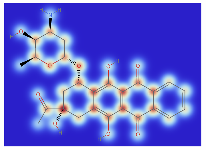
In their paper, Riniker and Landrum used a bivariate Gaussian for producing these heatmaps. One can instead use a number of other "blob" functions that are simpler to compute, yet give qualitatively similar results. Glassner gives a bunch of them here, but I have found the blob function by Baranoski and Rokne to be simple yet flexible enough for this application:
Make the appropriate modifications to the heatmap code, so that the Gaussians are replaced with the blob function:
One could also consider doing a 3D version of these heatmaps. For example, let's use the proteasome inhibitor ixazomib, and visualize its Gasteiger partial charges:
We slightly modify the tuning parameter for the blob function, and then use DensityPlot3D along with MoleculePlot3D to visualize the molecule along with its 3D heatmap:
Admittedly, making the 3D heatmap is a bit more fiddly than the 2D version, due to the need to tweak the blob parameters to get a reasonable picture. Some more work is needed to fully automate the adjustment of the blob, as well as the adjustment of the OpacityFunction to ensure only the appropriate parts of the molecule are accentuated by the 3D heatmap.
CITE THIS NOTEBOOK
CITE THIS NOTEBOOK
Molecular heatmaps via weighted Gaussian & rational-blob kernel summation over per-atom descriptors
by J. M.
Wolfram Community, STAFF PICKS, June 5, 2026
https://community.wolfram.com/groups/-/m/t/3727989
by J. M.
Wolfram Community, STAFF PICKS, June 5, 2026
https://community.wolfram.com/groups/-/m/t/3727989