A ball-bot is a vehicle that is balanced on a single spherical wheel and therefore has omnidirectional mobility. The ball-bot unique setup imbues it with special dynamic characteristics such as an negligibly small turning radius and the ability to change direction without the necessity to yaw. The control of a ball-bot robot is a complex and interesting problem since it is inherently unstable, as well as under-actuated: it has more degrees of freedom than independent control inputs. The ball is directly controlled by the control inputs while the body has no direct control over itself and is kept upright around its unstable equilibrium point by the control applied to the ball. In this example, the equations of motion are derived for the ball-bot and subsequently, a simulation and control is implemented on the model in order to stabilize it.
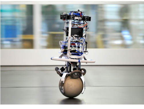
Modeling the Ball-bot Robot
Modeling the Ball-bot Robot
Legends and Parameters
Legends and Parameters
Symbol | Parameter/Variable | Value |
m B | massofbody | 10kg |
m b | massofball | 3kg |
ℐ B | momentofinertiaofbody | 4.76 2 kgm |
ℐ b | momentofinertialofball | 0.0239 2 kgm |
ℐ Bxy | momentofinertialofbodyinxy | 0.092 2 kgm |
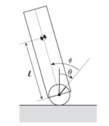
ℓ | fromcenterofmasstobodycenterofmass | 0.5m |
g | gravitationalacceleration | 9.8m/ 2 s |
r b | radiusofball | 0.06m |
θ | angleofballrotationwithrespecttotheverticalaxis | radians |
ϕ | anglebetweenverticalaxisandcenterofmass | radians |
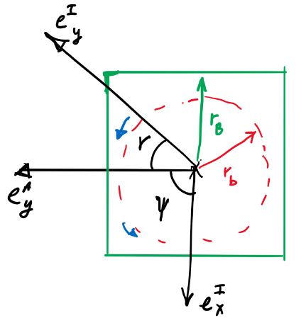
ψ | angleofballaroundverticalaxis | radians |
ν | angleofbodyaroundverticalaxis | radians |
i | drivetorqueinput | N/m |
b i | frictionfunction | N/m |
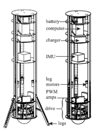
The parameters as a list of replacement rules:
In[]:=
pars={->10,->3,->0.125,->0.0239,->4.72,->0.092,ℓ->0.5,g->9.8};
m
B
m
b
r
b
ℐ
b
ℐ
B
ℐ
Bxy
Model Description
Model Description
The three-dimensional system is divided into three independent planar models, one in the -plane, one in -plane and one in the -plane resulting in a system with two degrees of freedom:
xy
yz
xy
◼
The rotation and translation of the ball
m
b
◼
The rotation of the body
m
B
The two planar models in the -plane and the in -plane the are treated as two independent identical models which alleviates the necessity to take into coupling account. The resulting systems are each independently similar to an inverted pendulum in each plane.
xy
yz
The states of the system are therefore taken to be the orientation angles θ, ψ for the ball and ϕ, ν for body along with their respective rates. The inputs to the system are the torques affecting the orientation angles.
1,2,3,4
Assumptions
Assumptions
The following assumptions where made during the modeling of the system for simplicity:
◼
No slippage: there is no slippage between the ball and the ground or between the ball and the torque wheels (actuators). Additionally, it is assumed that the torque applied is within a range where slippage will not occur.
◼
Friction: the friction between the ball and the body and between the ball and the floor is taken to be step function. This simplification is made due to the relatively small velocity and movement range of the robot.
◼
No deformation: it is assumed that the ball and actuators do not deform during the operation of the robot.
◼
Rapid motor dynamics: the responses of the motor are assumed to be much faster than the controller dynamics and therefore the motor torques can be assumed to be the inputs of the system.
◼
Ball movement constraints: it is assumed that the ball can only move on the horizontal plane. It cannot move vertically. Additionally, the robot will not traverse terrain with steep inclines.
Deriving the Equations of Motion in the xz and yz Planes:
Deriving the Equations of Motion in the and Planes:
xz
yz
The Lagrangian method is used to derive the equations of motion for system in each of the three planar models, each containing two degrees of freedom.
◼
Ball kinetic energy:
In[]:=
k
b
1
2
ℐ
b
2
θ'[t]
m
b
2
(θ'[t])
r
b
◼
Body kinetic energy:
In[]:=
k
B
m
B
2
2
r
b
2
θ'[t]
r
b
2
θ'[t]
2
ℓ
2
(θ'[t]+θ'[t])
ℐ
B
2
2
(θ'[t]+ϕ'[t])
◼
Ball potential energy:
In[]:=
b
◼
Body potential energy:
In[]:=
B
m
B
The Lagrangian is hence:
In[]:=
ℒ=(+)-(+)
k
b
k
B
B
b
Out[]=
-gℓCos[θ[t]+ϕ[t]]+[t]+[t]++4[t]+[t]+2ℓCos[θ[t]+ϕ[t]]([t]+[t][t])
m
B
1
2
m
b
2
r
b
2
′
θ
ℐ
b
2
′
θ
1
2
ℐ
B
2
([t]+[t])
′
θ
′
ϕ
1
2
m
B
2
ℓ
2
′
θ
2
r
b
2
′
θ
r
b
2
′
θ
′
θ
′
ϕ
The Euler-Lagrange equation yields the equations of motion in the and planes:
xz
yz
In[]:=
eqns=Table[D[ℒ,q'[t]]-D[ℒ,q[t]]==[t],{q,{θ,ϕ}}]/.[t]->[t]-0.015[t]θ'[t],[t]->[t]-0.02[t]ϕ'[t]
∂
t
q
θ
1
b
1
ϕ
2
b
2
Out[]=
-gℓSin[θ[t]+ϕ[t]]+ℓSin[θ[t]+ϕ[t]]([t]+[t][t])+2[t]+2[t]+([t]+[t])+-2ℓSin[θ[t]+ϕ[t]]([t]+[t])(2[t]+[t])+8[t]+2[t]+2ℓCos[θ[t]+ϕ[t]](2[t]+[t])[t]-0.015[t][t],-gℓSin[θ[t]+ϕ[t]]-ℓSin[θ[t]+ϕ[t]][t]([t]+[t])+ℓSin[θ[t]+ϕ[t]]([t]+[t][t])+ℓCos[θ[t]+ϕ[t]][t]+([t]+[t])[t]-0.02[t][t]
m
B
m
B
r
b
2
′
θ
′
θ
′
ϕ
1
2
m
b
2
r
b
′′
θ
ℐ
b
′′
θ
ℐ
B
′′
θ
′′
ϕ
1
2
m
B
r
b
′
θ
′
ϕ
′
θ
′
ϕ
2
ℓ
′′
θ
2
r
b
′′
θ
r
b
′′
θ
′′
ϕ
1
b
1
′
θ
m
B
m
B
r
b
′
θ
′
θ
′
ϕ
m
B
r
b
2
′
θ
′
θ
′
ϕ
m
B
r
b
′′
θ
ℐ
B
′′
θ
′′
ϕ
2
b
2
′
ϕ
The initial conditions satisfy the equilibrium point:
In[]:=
eqns/.{Derivative[_][_][t]:>0,[t]:>0,θ[t]:>0,ϕ[t]:>0}
Out[]=
{True,True}
Deriving the Equations of Motion in the xy plane:
Deriving the Equations of Motion in the plane:
xy
◼
Kinetic energy of the ball:
In[]:=
k
bxy
1
2
ℐ
b
2
ψ'[t]
◼
Kinetic energy of the body:
In[]:=
k
Bxy
1
2
ℐ
Bxy
2
ν'[t]
◼
The total potential energy for both the ball and the body are zero:
In[]:=
bxy
Bxy
The Lagrangian is hence:
In[]:=
ℒ
xy
k
bxy
k
Bxy
The Euler-Lagrange equation yields the equations of motion in the and planes:
xz
yz
In[]:=
eqns
xy
∂
t
ℒ
xy
ℒ
xy
q
ψ
3
b
3
ν
3
Out[]=
{[t][t]-[t][t],[t][t]}
ℐ
b
′′
ψ
3
b
3
′
ψ
ℐ
Bxy
′′
ν
3
The complete equations of the system:
In[]:=
eqns=Join[eqns,]
eqns
xy
Out[]=
-gℓSin[θ[t]+ϕ[t]]+ℓSin[θ[t]+ϕ[t]]([t]+[t][t])+2[t]+2[t]+([t]+[t])+-2ℓSin[θ[t]+ϕ[t]]([t]+[t])(2[t]+[t])+8[t]+2[t]+2ℓCos[θ[t]+ϕ[t]](2[t]+[t])[t]-0.015[t][t],-gℓSin[θ[t]+ϕ[t]]-ℓSin[θ[t]+ϕ[t]][t]([t]+[t])+ℓSin[θ[t]+ϕ[t]]([t]+[t][t])+ℓCos[θ[t]+ϕ[t]][t]+([t]+[t])[t]-0.02[t][t],[t][t]-[t][t],[t][t]
m
B
m
B
r
b
2
′
θ
′
θ
′
ϕ
1
2
m
b
2
r
b
′′
θ
ℐ
b
′′
θ
ℐ
B
′′
θ
′′
ϕ
1
2
m
B
r
b
′
θ
′
ϕ
′
θ
′
ϕ
2
ℓ
′′
θ
2
r
b
′′
θ
r
b
′′
θ
′′
ϕ
1
b
1
′
θ
m
B
m
B
r
b
′
θ
′
θ
′
ϕ
m
B
r
b
2
′
θ
′
θ
′
ϕ
m
B
r
b
′′
θ
ℐ
B
′′
θ
′′
ϕ
2
b
2
′
ϕ
ℐ
b
′′
ψ
3
b
3
′
ψ
ℐ
Bxy
′′
ν
3
In[]:=
eqns/.{Derivative[_][_][t]:>0,[t]:>0,[t]:>0,θ[t]:>0,ϕ[t]:>0,ψ[t]:>0,ν[t]:>0}
b
Out[]=
{True,True,True,True}
Controlling the Ball-bot
Controlling the Ball-bot
Now that we have the equations of motion that describe the dynamics of the system, we can proceed assess the open-loop response, in order to design and tune an adequate controller. Since the equations are nonlinear, we can use to obtain the most accurate model of the system. The number of states are the angles and the angular rates which describe the robot’s orientation and movement, the inputs feedback inputs are the torques and the disturbance inputs are the frictions. The outputs are the four angles describing the orientation.
The open-loop response:
The open-loop response:
Unsurprisingly, the response of the open-loop system is unstable for the xz- and yz-planes and unregulated for the xy-plane.
Designing a Linear Quadratic Gaussian Controller (LQG) for the system:
Designing a Linear Quadratic Gaussian Controller (LQG) for the system:
The design and implementation of the controller requires the specification of the feedback inputs. We can do that using a associations:
A set of regulator weights for the optimal regulator:
The optimal regulator controller data object:
A set of process and measurement noise covariance matrices for the optimal estimator:
The gains of the optimal estimator:
The LQG regulator can now be assembled using the optimal regulator and the optimal estimator gains:
Using the same initial conditions as before, the output response of the closed-loop system with the LQG in the feedback path indicates the states are now regulated:
While the controlled system has a satisfactory performance, it is important to asses the control effort. If the control effort requires an unreasonable amount of energy, the system is unfeasible! We can assess the control signal by measuring the controller’s signal to the plant. We start by obtaining the controller model from the controller data-object via it’s corresponding property:
The output response of the controller model with the state response as the input will yield the control signals for each of the 4 inputs: