CITE THIS NOTEBOOK: Diagrammatic and computational study of Abrikosov vortex interactions by Gianni Tallarita. Wolfram Community JAN 11 2023.
ORIGINAL ARTICLE: Eto, M., Peterson, A., Schaposnik Massolo, F.I. et al. Dynamics of global and local vortices with orientational moduli. J. High Energ. Phys. 2021, 156 (2021). https://doi.org/10.1007/JHEP03(2021)156.
ORIGINAL ARTICLE: Eto, M., Peterson, A., Schaposnik Massolo, F.I. et al. Dynamics of global and local vortices with orientational moduli. J. High Energ. Phys. 2021, 156 (2021). https://doi.org/10.1007/JHEP03(2021)156.
Abrikosov vortices are topological solitons of the Ginzburg-Landau action. The solutions they describe are abundant in nature: type II superconductors in condensed matter, cosmological strings in the early universe, flux tubes in confinement mechanisms in QCD, etc. While a lot is known about the asymptotic states of their scattering processes, little is known about the bound states they form when they are at the closest point of interaction. This project wishes to begin studying these interaction moments systematically through a diagrammatic classification of the space-time events in 2d vortex systems. We construct the space-time diagram of vortex trajectories, paying particular attention to the intermediate states corresponding to vortex interactions.
IMPORTANT NOTE : The coding previous to the precise goal of this project was done in a separate notebook and, for length reasons, is not copied here . This is the code that led to the publication [1] and which we refer to here as “Theoretical setting and Numerical Method” section . We describe in the part referring to that section a broad summary of what this previous code does. We then extend this code to produce the new results of this project at the end of this notebook, in the section we refer to as “Space-time diagrams and intermediate states”. Also, successful implementation of the functions loaded in this notebook relies on separately stored data of runs.
Theoretical setting and Numerical Method
Theoretical setting and Numerical Method
Theoretical Introduction
Theoretical Introduction
Superconductivity is the phenomenon of electric flow without resistance. It occurs in specific kinds of metals below critical temperatures and is key to many of the most incredible technological applications of modern society (for example, the Large Hadron collider has superconducting magnets in order to keep protons on collision tracks). The nucleus of atoms contains protons and neutrons, these in turn are made of smaller particles called quarks. Quarks confine, meaning that a single isolated quark cannot be found in nature (at our normal energy scales). They only occur in pairs or triplets (more recently tetraplets and pentaplets were also found!). Why do they confine? No-one knows. Answering this question will award the person who solves it a Nobel prize. These are seemingly completely unrelated topics, but in fact they are not: both contain Abrikosov vortices at the very center of their physics. At low energies, these vortices are described by the Ginzburg - Landau Lagrangian.
The Ginzburg-Landau Lagrangian admits static, vortex solutions corresponding to windings of the U(1) symmetry on the circle at infinity. This Lagrangian is the following,
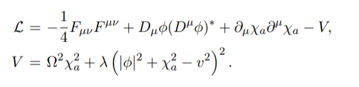
where F describes the electromagnetic field strength tensor, ϕ is the Higgs field, χ is a real triplet of scalar fields and V is the interaction potential. Note that ϕ is coupled to the electromagnetic field A via the covariant derivative Dϕ. Therefore, this system describes a Higgs field interacting with electromagnetism. Note that the potential is a quartic, symmetry breaking potential meaning that this Lagrangian has spontaneous symmetry breaking. The parameter v is the vacuum expectation value of the Higgs field, i.e. the value the field takes in the vacuum. λ is a parameter which controls the width of the vortex solution and Ω is a frequency parameter for the χ field.
These vortices are Solitonic solutions of the equations of motion of the above Lagrangian, Solitonic meaning they are finite, classically sized lumps of energy . In this case, these solitons are topological, in the sense that they are stabilised by the topological winding at infinity . Finding these static, cylindrically symmetric solutions is a simple ODE numerical problem. It boils down to the following system of equations:
These vortices are Solitonic solutions of the equations of motion of the above Lagrangian, Solitonic meaning they are finite, classically sized lumps of energy . In this case, these solitons are topological, in the sense that they are stabilised by the topological winding at infinity . Finding these static, cylindrically symmetric solutions is a simple ODE numerical problem. It boils down to the following system of equations:
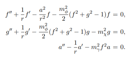
where f is the modulus of the Higgs field, g is the modulus of the χ field and a is the electromagnetic vector potential in the θ direction on the cylindrical plane . All fields here depend on the radial coordinate r only .
I solve these solutions by a spatial discretization of the radial line, using finite differences for derivatives and then the magic FindRoot function in Mathematica . Solutions look like this :

I show only the f profile of the Higgs field above . Note that this tends to v (in this case v=2), the vacuum expectation value present in the potential, at infinity and goes to 0 at the origin of the plane . The region where f is distinctly different from v is the vortex solution . Inside this region the magnetic field is maximum and outside it quickly goes to zero : the so called Meissner effect .
The idea now is to study how these objects interact with themselves . In order to do this, we take these solutions and Lorentz boost them towards each other letting them collide. Thefore the same field solution is made dynamic by the Lorentz boost. In order to evolve the system we must solve the evolution equations:
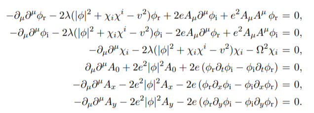
These equations are solved numerically using a 4th order Runge Kutta procedure, as detailed in the next section .
Numerical Approach, long live GPUs!
Numerical Approach, long live GPUs!
While the default function NDSolve does have a built - in RK procedure, I found that this wasn't sufficient to solve this problem . Furthermore, it relies on CPU computation, which is painfully slow when dealing with large grid systems .
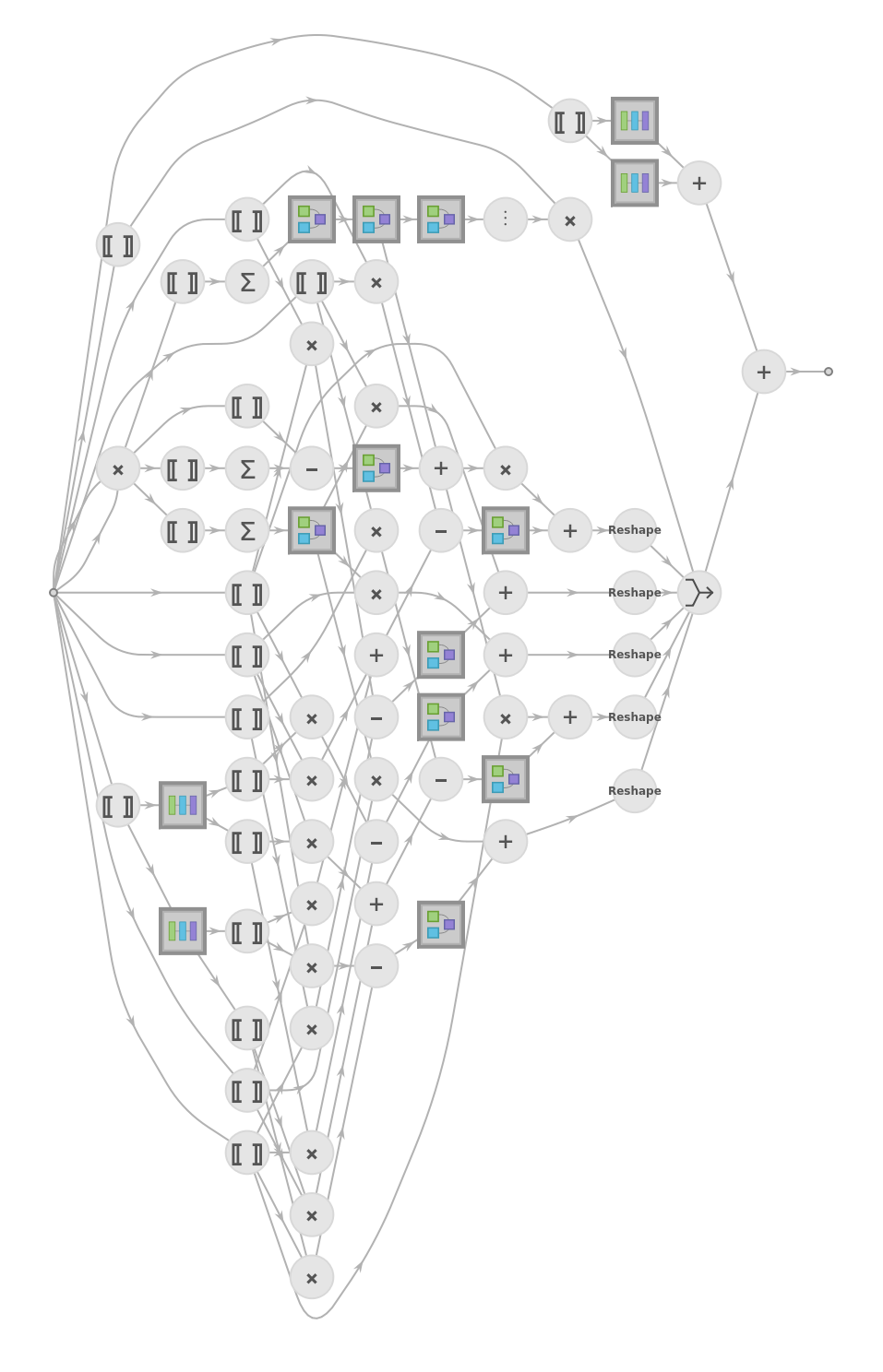
Therefore, I decided to code my own system of evolution using the Neural Network formalism built into Mathematica . While this makes actual equation implementation fairly painful, the massive advantage is that it allows one to work with GPUs, which for this specific problem gives a speed boost of around 130. This means a computation that on CPU takes 1 day is now reduced to roughly 10 minutes .
Written in Neural Graph format, the above evolution equations look like this :
Out[]=
NetGraph



WhilethestandardRK4procedure,whichwecanreadofffromWikipedia[2]
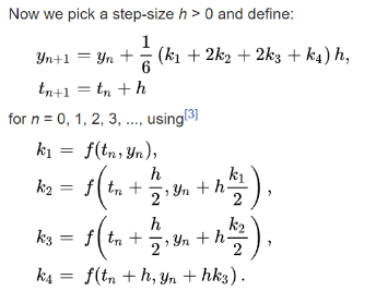
becomes
NetGraph
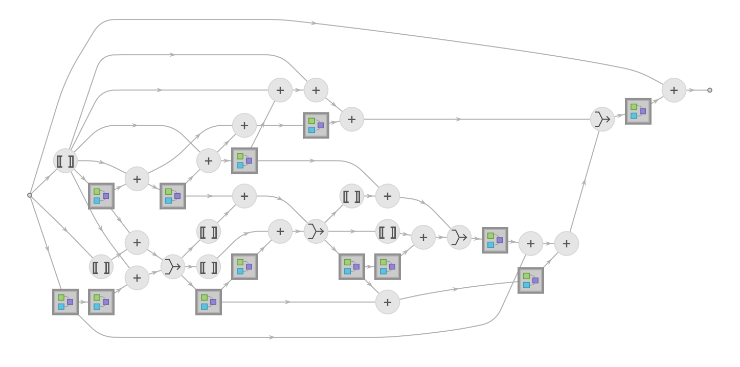
This RK4 algorithm is then looped on using the (amazing!) function NetNestOperator. A specific example of a possible scattering outcome is represented by the following figure, which shows the energy profile of two vortices colliding and scattering:
For all details of the above setup I refer the reader to [1].
The main problem, to which this project is dedicated, is the study of the intermediate vortex interaction states of these vortices. This would be roughly the moment shown by the third and middle snapshot shown above, when the vortices are at maximal interaction. Why is this a problem? Because very little is known about the physics of these moments. What is generally done is just to solve the equations numerically, but no real analytical control of what happens there is known. In fact, no real study of long lived intermediate states is known at all. When vortices meet, they form intermediate bound states which have a life and physics of their own, and not much is known about it. What this project initiates is a study of precisely this part of the vortex interaction. The method is construct space-time Contour diagrams of these interactions in order to then do image post-processing on the intermediate bound states. This is only partially achieved below, I was able to construct these diagrams, some of which are incredible interesting, but the image post-processing is a complex process of which I only scratch the surface.
The main problem, to which this project is dedicated, is the study of the intermediate vortex interaction states of these vortices. This would be roughly the moment shown by the third and middle snapshot shown above, when the vortices are at maximal interaction. Why is this a problem? Because very little is known about the physics of these moments. What is generally done is just to solve the equations numerically, but no real analytical control of what happens there is known. In fact, no real study of long lived intermediate states is known at all. When vortices meet, they form intermediate bound states which have a life and physics of their own, and not much is known about it. What this project initiates is a study of precisely this part of the vortex interaction. The method is construct space-time Contour diagrams of these interactions in order to then do image post-processing on the intermediate bound states. This is only partially achieved below, I was able to construct these diagrams, some of which are incredible interesting, but the image post-processing is a complex process of which I only scratch the surface.
Space-time diagrams and intermediate states
Space-time diagrams and intermediate states
Now we want to construct space time evolution diagrams of these vortex collisions to study their interaction states
The above is a directory for the simulation data of vortex collisions . This data can be made available to the reader upon requested .
Next, we need a two dimensional grid for the numerical system .
Extracting Vortex position Data
Extracting Vortex position Data
While the data above contains the evolution of the whole fields, we ideally want to be able to track the positions of the vortex cores only . This will give us a good idea of how to then construct centroid diagrams, which is what I did first .
The VortexData function is a function that given a simulation, tracks the coordinate positions of the centers of the vortices only
Lets try and apply this to a vortex scattering of the form shown in the bottom figure of the first section of this notebook
First, let' s make sure we put all simulation files in termporal order
Then, we need to apply a norm between vortex positions at different time snapshots, or the VortexData function get' s confused as to which vortex is which in the scattering process
The result of the whole process are the pictures above . We see here two plots corresponding to the positions of the vortices in the x - direction vs time (first plot), and y - coordinate vs time (below plot) . We can trace back this plot to the figure in the first section. Vortices advance in the x direction, meet, interact, and come out in the y-direction. Note the correct tracking of each vortex, without the norm procedure above the two lines would mix colours.
Centroid Diagrams
Centroid Diagrams
The above algorithm allows us to construct the simplest space - time diagram possible, that is the centroid diagrams, which are just 3 d diagrams of the vortex positions using the time coordinate as a "z" axis. This is achieved using the ParametricPlot3D function. What the code below does is therefore to take the vortex data and append the time coordinate as a z-axis, which is then plotted parametrically.
The above diagram is the result of this procedure for the scattering process we are now familiar with . Note that, as shown below, this code works perfectly with more vortices than just two. I tried with a scattering simulation of 4 -vortices as well.
Space - Time Contour Diagrams
Space - Time Contour Diagrams
The above diagrams, while a concrete step in the right direction, don' t reveal anything about the interaction states of vortices . Therefore, we need a more powerful form of diagram to be able to see these states . This is what this section does . In practice, the way to achieve this is to generalise the above results to plotting the evolution of the whole contours of the fields, rather than just the center of the vortices .
The process is computationally expensive, therefore we introduce a skip parameter in order to make calculations faster . The skip parameter skips the nth frame of the simulation data .
Finally, we use the ListContourPLot3D function to visualize the system . One has to massage the graphics option of this function considerably in order to have plots that make sense . The key ingredient is to pick the MaxPlotPoints appropriately .
The above plot is one that can be generated in roughly 5 minutes of processing . While it is clearly the correct plot, it looks awful . Therefore what I did next is to let the system evolve with full accuracy . This takes hours, therefore I let many of these run over night . The results are shown in the next section .
A Bestiary of Vortex interactions
A Bestiary of Vortex interactions
This is a catalogue of vortex interaction space - time diagrams with high accuracy . A brief description is added to the title of each case. I say if the scattered vortices are repulsive or attractive to begin with (this depends on the specif choice of parameters in the Lagrangian), I also included at what velocity, as a fraction of the speed of light, these vortices are boosted towards each other.
repulsive, v = 0.8. This is the familiar case shown above we have been working with most of the project
repulsive, v = 0.8. This is the familiar case shown above we have been working with most of the project
repulsive, v = 0.4
repulsive, v = 0.4
Image recognition- The beginning of post-production analysis
Image recognition- The beginning of post-production analysis
As can be seen, we see many exotic intermediate states of vortex interactions . These are what we have to study in order to extract some important physical information . This section begins the image postprocessing analysis in order to see if one can extract information from the above diagrams. In thise section we never get to the 3d image processing needed for the previous diagrams. What we achieve is a 2d tracking of vortex positions just from the contour diagrams.
Using the PixelValuePositions function we identify the regions of each 2 d plot corresponding to the center of the vortices . This is the equivalent of the vortexdata function but diagramatically!
Here I display on the 2 d diagram the highlighted positions of the vortices in white colour, we see that the function works nicely .
Finally, by clustering the vortices in terms of the number of vortices, I try to diagramatically construct the trajectory of a specific vortex through time, just by tracking the white colours in the 2 d plots .
We see that the algorithm works, showing us the trajectory of a specific vortex through time only through image analysis . One would have to extend this to the full 3 d contour case using Image3D postprocessing tools . I wasn' t able to achieve this in the given time .
Concluding remarks
Concluding remarks
In this project I constructed the space time diagrams of vortex interactions, gathering the data of previous vortex scattering simulations. Initially, I made centroid diagrams which are just the space-time diagrams corresponding to tracking the center position of the vortices only. Then, I extended this to the full Contour diagrams. These diagrams are computationally expensive to construct, so there might be a better way to do so. Importantly, the interaction sections of these diagrams are the first 3d renderings of vortex intermediate states. An in-depth analysis of these states, involving Opacity functions and 3d Image post-processing should be done next in order to extract relevant physical knowledge of the system.
Keywords
Keywords
◼
[Soliton]
◼
[Vortex]
◼
[Scattering]
◼
[GPU]
Acknowledgment
Acknowledgment
I kindly acknowledge my tutor Brad Klee and Stephen Wolfram for creating this interesting project.
References
References