Introduction
Introduction
Consider the following finite, square grid and triangle:
In[]:=
$EQ = "";eqRow[args__] := Panel@Row[{args}, $EQ]pgrid[args__] := Panel@Grid[args]prow[args__] := Panel@Row[args]labelPos[snap:{lo1_, hi1_}, loc:{lo2_, hi2_}] := With[ {tests = TrueQ/@{lo1≤lo2, hi1≤hi2}}, snap + .2 * (tests /. {True-1, False1})]DynamicModule[ {grid = Flatten[Table[{i, j}, {i, -5, 5}, {j, -5, 5}], 1], A, B, C, a, b, c, min = -5, max = 5}, Manipulate[ {a, b, c} = Flatten[Nearest[grid, #, 1]& /@ {A, B, C}, 1]; Panel[Column[ Show[ Graphics[ Directive[EdgeForm@Blue, Yellow], Triangle[{a, b, c}], Black, Text["A", labelPos[a, A]], Text["B", labelPos[b, B]], Text["C", labelPos[c, C]] , ImageMargins5, PlotLabel"Can you find an equilateral triangle whose vertices are lattice points?" ], ListPlot[grid, AspectRatio1, PlotStyleDarker@Green] , ImageSizeLarge, AxesTrue, Ticks({#, #}& @ Table[i,{i,-5,5}]) ], Column[ Row[ eqRow["{,}", a], eqRow["{,}", b], eqRow["{,}", c] , Spacer[5] ], pgrid@ {TraditionalForm[Abs["AB"]], $EQ, #, " ≈ ", N@#}&[Norm[a-b]], {TraditionalForm[Abs["AC"]], $EQ, #, " ≈ ", N@#}&[Norm[a-c]], {TraditionalForm[Abs["BC"]], $EQ, #, " ≈ ", N@#}&[Norm[b-c]] ] , Center ]], {{A, {0, -2}}, Locator}, {{B, {1, 2}}, Locator}, {{C, {-3, 1}}, Locator}, AppearanceElementsNone, PaneledFalse ], SaveDefinitionsTrue]
A
1
A
2
B
1
B
2
C
1
C
2
Out[]=
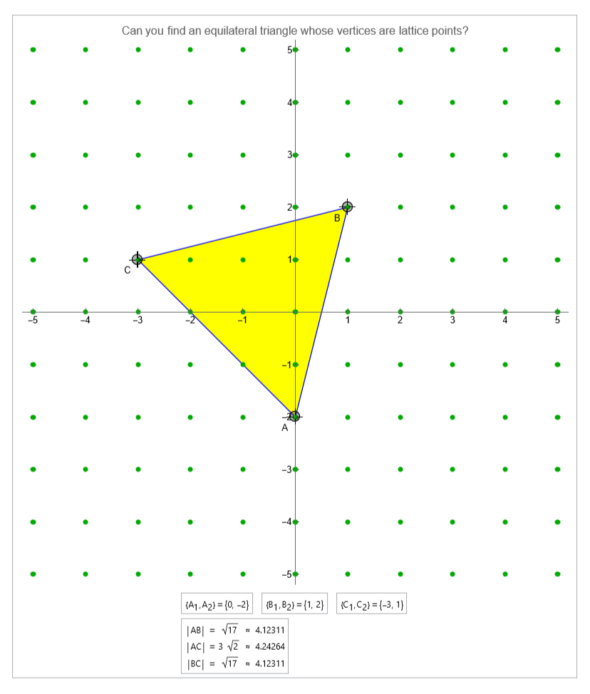
The yellow triangle looks equilateral, but the side lengths displayed below the plot tell a different story — it is only isosceles — with the edge AC being slightly longer than the remaining two edges. Feel free to play around with the positions of the vertices A, B, and C and try to see if you can find a configuration which gives an equilateral triangle. It shouldn’t take too long to convince yourself that this is an impossible task, at least when you constrain yourself to such a small grid. But maybe, if we were working with a larger grid, it might be possible to find an equilateral triangle? In this demonstration we answer this question in the negative - no matter the size of the grid, no regular polygon other than a square can have all vertices coincide with points on a grid.
Visualizing Lattices and their Properties
Visualizing Lattices and their Properties
We introduce some standard mathematical language which will hopefully make the ideas presented in this notebook easier to follow and understand. An (integer) lattice in n-dimensional space we will mean the collection of points . Simply put these are points in n-dimensional space whose coordinates are integers. We’ve already shown what this looks like in 2 dimensions, and here’s part of a 3-dimensional lattice:
{(,,...,)∈:,,...,∈}
x
1
x
2
x
n
n
x
1
x
2
x
n
In[]:=
latticeSlice[x_:5, y_:5, z_:5] := ListPointPlot3D[Flatten[Table[{i, j, k}, {i, -x, x}, {j, -y, y}, {k, -z, z}], 2], AspectRatio 1, Axes True, Boxed False, PlotStyle Darker[Green], PlotLabel "A lattice in 3 dimensions"]Rasterize@latticeSlice[]
Out[]=
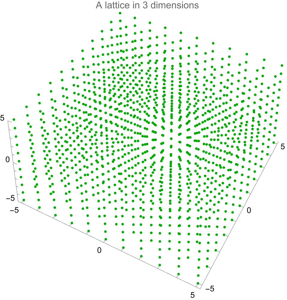
In dimensions 4 and higher visualizing the lattice becomes impossible, but the same rules apply — lattice points are points with integer coordinates. From now on when talking about a lattice we will specifically mean the 2-dimensional lattice. In this particular case lattice points have what is know as a ring structure, that is they can be added and multiplied and the result of these operations is again a lattice point. The formulae for addition and multiplication are as follows: • ; • . Notice that if the coordinates on the left hand side are integers, then so are the coordinates on the right hand side. The multiplication formula may seem a bit mysterious if you hadn’t encountered it before, however if you’ve taken a course in Complex Analysis you’ll recognize that it is exactly the rule for multiplication of complex numbers. More formally we can say that our lattice is a sub-ring of the field of complex numbers. If this sounds arcane don’t worry — all we really need to know is that we can add points and that multiplying a point by is equivalent to rotating it 90° counterclockwise around the origin, as can be seen below. Using this tool we can actually rotate a point 90° about any other point as well.
(,)+(,)=(+,+)
x
1
y
1
x
2
y
2
x
1
x
2
y
1
y
2
(,)(,)=(-,+)
x
1
y
1
x
2
y
2
x
1
x
2
y
1
y
2
x
1
y
2
x
2
y
1
(0,1)
The Case of the Equilateral Triangle
The Case of the Equilateral Triangle
To prove that no three lattice points determine an equilateral triangle we argue by contradiction. Assume there exists an equilateral triangle with side length L whose vertices belong to a lattice. As mentioned before, we are free to assume that one vertex of the triangle, denoted by O, lies at the origin:
For our next step we make use of the fact that we can rotate points. Rotating each vertex of the hexagon 90° around its counterclockwise neighbor yields a new, smaller, but still regular hexagon. We are also guaranteed that the vertices of the smaller hexagon are lattice points.
What About Other Regular Polygons?
What About Other Regular Polygons?
So far we’ve demonstrated that we cannot find an equilateral triangle or a regular hexagon whose vertices are lattice points. It turns out that the same construction that worked for hexagons works for almost all other regular polygons. Below we demonstrate the shrinking procedure for pentagons and heptagons.
We need the coordinates of c to figure out where the shrinking procedure will send b.
Let us denote the square of the length of the side of our n-gon by L. Clearly L is equal to the square of the distance between two consecutive vertices of our n-gon.
The n-gon shrinking process takes each vertex p to a new vertex p’. To find the shrinking factor ρ(n) we first compute L’ — the square of the side length of the shrunk n-gon.
With this we have found the general formula for the square of the length of the side of the shrunk n-gon:
This seems quite complicated, but Simplifying the formula yields something much more tractable:
Now let’s see which values of n result in ρ being less than 1:
Let’s see what the shrinking procedure looks like:
Further Reading
Further Reading
If you found this theorem interesting and would like to learn about more similar results I recommend the following articles:
• Klamkin, M. and Chrestenson, H. E. “Polygon Imbedded in a Lattice.” Amer. Math. Monthly 70, 51-61, 1963.
• http://dynamicsofpolygons.org/PDFs/LatticePolygons.pdf
• Klamkin, M. and Chrestenson, H. E. “Polygon Imbedded in a Lattice.” Amer. Math. Monthly 70, 51-61, 1963.
• http://dynamicsofpolygons.org/PDFs/LatticePolygons.pdf