Collision integrals versus dimensionless temperature
Housam Binous and Ahmed Bellagi
Collision integrals versus dimensionless temperature
Housam Binous and Ahmed Bellagi
Housam Binous and Ahmed Bellagi
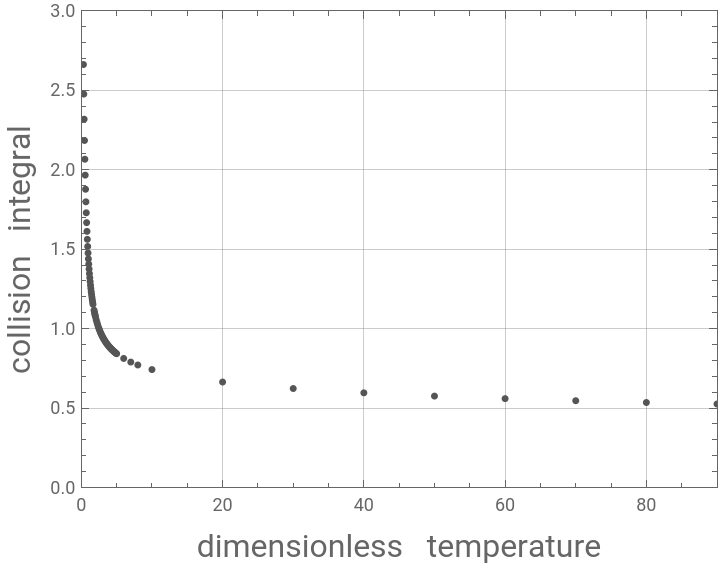
The collision integrals, (for mass diffusivity) and = (for thermal conductivity and viscosity), are computed based on the Lennard–Jones potential.Collision integrals are dimensionless functions of the temperature and of the intermolecular potential field for one molecule of A and one molecule of B.Appendix K of Ref. 1 tabulates values of and =, as a function of κ×T / where κ is the Boltzmann constant, equal to 1.38 ergs/K, and is the energy of molecular interaction for the binary system A and B, a Lennard–Jones parameter, in ergs.Neufeld and coworkers (Ref. 2) developed empirical equation in order to provide estimates of these collision integrals. Such equation makes computerized calculations more convenient.=A×+C×+E×+G×and==A×+C×+E×+G×-R××Sin(P-S×)where Here, we use NonlinearModelFit in order to fetch new sets of the empirical constants that yield slightly smaller sum of squared residuals.References :[1] J. R. Welty, G. L. Rorrer and D. G. Foster, Fundamentals of Momentum, Heat, and Mass Transfer, 7th Edition, NY: Wiley, 2019.[2] P. D. Neufeld, A. R. Janzen, and R. A. Aziz, J. Chem. Phys., 57, 1100 (1972).
Ω
D
Ω
k
Ω
μ
Ω
D
Ω
k
Ω
μ
ϵ
AB
-16
10
ϵ
AB
Ω
D
-B
TS
-D×TS
-F×TS
-H×TS
Ω
k
Ω
μ
-B
TS
-D×TS
-F×TS
-H×TS
B
TS
W
TS
TS=κ×T/
ϵ
AB
Ω
D
-B
TS
-D×TS
-F×TS
-H×TS
In[]:=
Clear[A1,B1,C1,D1,E1,F1,G1,H1,R1,S1,W1,P1]
In[]:=
OMEGA11=A1/TS^B1+C1/Exp[D1TS]+E1/Exp[F1TS]+G1/Exp[H1TS]
Out[]=
C1+E1+G1+A1
-D1TS
-F1TS
-H1TS
-B1
TS
In[]:=
data={{0.3,2.662},{0.35,2.476},{0.4,2.318},{0.45,2.184},{0.5,2.066},{0.55,1.966},{0.6,1.877},{0.65,1.798},{0.7,1.729},{0.75,1.667},{0.8,1.612},{0.85,1.562},{0.9,1.517},{0.95,1.476},{1.,1.439},{1.05,1.406},{1.1,1.375},{1.15,1.346},{1.2,1.32},{1.25,1.296},{1.3,1.273},{1.35,1.253},{1.4,1.233},{1.45,1.215},{1.5,1.198},{1.55,1.182},{1.6,1.167},{1.65,1.153},{1.8,1.116},{1.85,1.105},{1.9,1.094},{1.95,1.084},{2.,1.075},{2.1,1.057},{2.2,1.041},{2.3,1.026},{2.4,1.012},{2.5,0.9996},{2.6,0.9878},{2.7,0.977},{2.8,0.9672},{2.9,0.9576},{3.,0.949},{3.1,0.9406},{3.2,0.9328},{3.3,0.9256},{3.4,0.9186},{3.5,0.912},{3.6,0.9058},{3.7,0.8998},{3.8,0.8942},{3.9,0.8888},{4.,0.8836},{4.1,0.8788},{4.2,0.874},{4.3,0.8694},{4.4,0.8652},{4.5,0.861},{4.6,0.8568},{4.7,0.853},{4.8,0.8492},{4.9,0.8456},{5.,0.8422},{6.,0.8124},{7.,0.7896},{8.,0.7712},{10.,0.7424},{20.,0.664},{30.,0.6232},{40.,0.596},{50.,0.5756},{60.,0.5596},{70.,0.5464},{80.,0.5352},{90.,0.5256}};(*datafromappendixKofRef.1*)
In[]:=
p1=ListPlot[data,Frame->True,GridLines->Automatic,AspectRatio->0.75,ImageSize->Medium,FrameLabel->{Style["dimensionless temperature",16],Style["collision integral",16]},PlotStyle->Darker@Gray,PlotRange->{{0,90},{0,3}}]
Out[]=
In[]:=
mdl=NonlinearModelFit[data,OMEGA11,{A1,B1,C1,D1,E1,F1,G1,H1},TS]
Out[]=
FittedModel
In[]:=
sol=Normal@mdl
Out[]=
1.63583+1.21352+0.284661+
-4.45147TS
-1.8126TS
-0.599496TS
1.06612
0.157468
TS
In[]:=
mdl["ParameterTable"]
Out[]=
Estimate | Standard Error | t-Statistic | P-Value | |
A1 | 1.06612 | 0.00114345 | 932.372 | 1.57477× -139 10 |
B1 | 0.157468 | 0.000301141 | 522.906 | 1.05414× -122 10 |
C1 | 1.63583 | 0.03284 | 49.8121 | 1.14103× -54 10 |
D1 | 4.45147 | 0.075705 | 58.8001 | 2.17399× -59 10 |
E1 | 1.21352 | 0.0296889 | 40.8744 | 4.26357× -49 10 |
F1 | 1.8126 | 0.0420876 | 43.0673 | 1.45906× -50 10 |
G1 | 0.284661 | 0.0137204 | 20.7472 | 7.08289× -31 10 |
H1 | 0.599496 | 0.015775 | 38.0029 | 4.60085× -47 10 |
In[]:=
A1N=1.06036;B1N=0.15610;C1N=0.19300;D1N=0.47635;E1N=1.03587;F1N=1.52996;G1N=1.76474;H1N=3.89411;(*constantsfromRef.2*)
In[]:=
{A1New,B1New,C1New,D1New,E1New,F1New,G1New,H1New}={1.06612,0.157468,1.63583,4.45147,1.21352,1.8126,0.284661,0.599496}(*constantsobtainedusingNonlinearModelFit*)
Out[]=
{1.06612,0.157468,1.63583,4.45147,1.21352,1.8126,0.284661,0.599496}
In[]:=
Grid[Transpose@{{" ","A","B","C","D","E","F","G","H"},{"Our Fit ",A1New,B1New,C1New,D1New,E1New,F1New,G1New,H1New},{"Ref. 1 ",A1N,B1N,C1N,D1N,E1N,F1N,G1N,H1N}},Background->{None,{Lighter[Yellow,.5],{White,Lighter[Blend[{Blue,Green}],.6]}}},Frame->All,ItemStyle->12,Spacings->{1.5,1.5}]
Out[]=
Our Fit | Ref. 1 | |
A | 1.06612 | 1.06036 |
B | 0.157468 | 0.1561 |
C | 1.63583 | 0.193 |
D | 4.45147 | 0.47635 |
E | 1.21352 | 1.03587 |
F | 1.8126 | 1.52996 |
G | 0.284661 | 1.76474 |
H | 0.599496 | 3.89411 |
Our fit has a lower sum of squared residuals
In[]:=
ourfit=Sum[(data[[i]][[2]]-sol)^2/.TS->data[[i]][[1]],{i,1,Length[data]}]
Out[]=
0.0000128369
In[]:=
fitNeufeld=Sum[(data[[i]][[2]]-(A1N/TS^B1N+C1N/Exp[D1NTS]+E1N/Exp[F1NTS]+G1N/Exp[H1NTS]))^2/.TS->data[[i]][[1]],{i,1,Length[data]}]
Out[]=
0.000250318
In[]:=
res=mdl["FitResiduals"];
In[]:=
Sum[res[[i]]^2,{i,1,Length[data]}]
Out[]=
0.0000128369
In[]:=
mdl["ANOVATableSumsOfSquares"][[2]]
Out[]=
0.0000128369
Ω
k
Ω
μ
-B
TS
-D×TS
-F×TS
-H×TS
B
TS
W
TS
In[]:=
Clear[A1,B1,C1,D1,E1,F1,G1,H1,R1,S1,W1,P1]
In[]:=
OMEGA22=A1/TS^B1+C1/Exp[D1TS]+E1/Exp[F1TS]+10^-4R1TS^B1Sin[S1TS^W1-P1]
Out[]=
C1+E1+A1-
-D1TS
-F1TS
-B1
TS
R1Sin[P1-S1]
B1
TS
W1
TS
10000
In[]:=
data={{0.3,2.785},{0.35,2.628},{0.4,2.492},{0.45,2.368},{0.5,2.257},{0.55,2.156},{0.6,2.065},{0.65,1.982},{0.7,1.908},{0.75,1.841},{0.8,1.78},{0.85,1.725},{0.9,1.675},{0.95,1.629},{1.,1.587},{1.05,1.549},{1.1,1.514},{1.15,1.482},{1.2,1.452},{1.25,1.424},{1.3,1.399},{1.35,1.375},{1.4,1.353},{1.45,1.333},{1.5,1.314},{1.55,1.296},{1.6,1.279},{1.65,1.264},{1.7,1.248},{1.8,1.221},{1.85,1.209},{1.9,1.197},{1.95,1.186},{2.,1.175},{2.1,1.156},{2.2,1.138},{2.3,1.122},{2.4,1.107},{2.5,1.093},{2.6,1.081},{2.7,1.069},{2.8,1.058},{2.9,1.048},{3.,1.039},{3.1,1.03},{3.2,1.022},{3.3,1.014},{3.4,1.007},{3.5,0.9999},{3.6,0.9932},{3.7,0.987},{3.8,0.9811},{3.9,0.9755},{4.,0.97},{4.1,0.9649},{4.2,0.96},{4.3,0.9553},{4.4,0.9507},{4.5,0.9464},{4.6,0.9422},{4.7,0.9382},{4.8,0.9343},{4.9,0.9305},{5.,0.9269},{6.,0.8963},{7.,0.8727},{8.,0.8538},{10.,0.8242},{20.,0.7432},{30.,0.7005},{40.,0.6718},{50.,0.6504},{60.,0.6335},{70.,0.6194},{80.,0.6076},{90.,0.5973}};(*datafromappendixKofRef.1*)
Our fit has a lower sum of squared residuals