The Wolfram Emerging Leaders Program: High School (WELP:HS) is a remote, semester-long program designed for exceptional graduates from the Wolfram High School Summer Research Program to continue to develop their skills. Students work in a small group over the course of a semester to do either a research-based project or a product development–based project under the guidance of expert mentors. Projects are centered around a topic at the intersection of the group’s interests.
This essay was written by:
This essay was written by:
This project presents a comprehensive analysis of the spread of trachoma in prevalent countries, focusing on Ethiopia and South Sudan, through the application of various Susceptible-Infectious-Recovered (SIR) model variations and community graph analyses. By combining different modeling methods, our project seeks to improve how well we can predict the spread of trachoma and understand the complicated interactions among different factors that affect how the disease is transmitted over time.
Introduction
Introduction
Trachoma, caused by the bacteria Chlamydia trachomatis, is a leading cause of preventable blindness globally, with symptoms ranging from eye irritation to eventual blindness if left untreated. Trachoma control and elimination efforts have made significant progress in recent years, but challenges persist, particularly in regions with limited resources. Responsible for the visual impairment of over 2 million individuals and blindness in more than 1.2 million people worldwide, trachoma remains a pressing public health issue. The disease spreads through contact with eye discharge from infected individuals and flies that carry the bacteria, accelerating transmission, especially in impoverished areas. Trachoma’s impact extends beyond individual suffering, affecting communities and worsening existing health inequities.
SIR (Susceptible-Infectious-Recovered)
SIR (Susceptible-Infectious-Recovered)
Introduction and Overview
Introduction and Overview
The SIR model, also known as the Kermack-McKendrick model, is the simplest of many models used to simulate the spread of infectious diseases, such as trachoma, within a population. SIR is an acronym for Susceptible-Infectious-Recovered, which are the three “compartments” each individual of a population can be classified under. The model utilizes a mathematical framework consisting of three ordinary differential equations, one for each compartment. Within the equations themselves, mathematical relationships are established that represent the rate of the population’s movement between each compartment with respect to each time step.
This model, and the others we will explore in this project, will allow people to estimate the impact of mitigation strategies such as vaccination and social distancing, as well as the general behavior of diseases such as trachoma over time. Although no model can perfectly simulate the real world, using them allows us to obtain a general overview of the dynamics of trachoma.
Defining Initial Constants and Rate Constants
Defining Initial Constants and Rate Constants
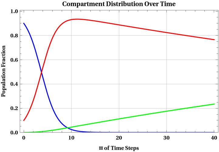
Instead of using actual population numbers, each constant represents the fraction of the total population in that compartment. Thus, the sum of the number of people in each compartment will always equal to 1 .0= susceptible + infectious + recovered
Constants to represent initial population values
In[]:=
susceptibleInitial=0.9infectiousInitial=0.1recoveredInitial=0.0
Out[]=
0.9
Out[]=
0.1
Out[]=
0.
Constants to represent rate transitions (based on actual rates of trachoma) and the number of time steps to run the simulation
In[]:=
infectRate=0.6recoveryRate=0.0074time=40
Out[]=
0.6
Out[]=
0.0074
Out[]=
40
Establishing and Solving for the Set of Ordinary Differential Equations
Establishing and Solving for the Set of Ordinary Differential Equations
With the constants set, we can create our set of differential equations for each compartment. Each differential equation is set to a single variable and consist of their integral counterpart (the actual number of people in that compartment).
In[]:=
eqS=sus'[t]==-infectRate*sus[t]*inf[t]eqI=inf'[t]==infectRate*sus[t]*inf[t]-recoveryRate*inf[t]eqR=rec'[t]==recoveryRate*inf[t]
Out[]=
′
sus
Out[]=
′
inf
Out[]=
′
rec
Using the NDSolve function, solutions are found to the set of differential equations with the specified initial values for the susceptible, infectious, and recovered compartments.
In[]:=
solutions=NDSolve[{eqS,eqI,eqR,sus[0]==susceptibleInitial,inf[0]==infectiousInitial,rec[0]==recoveredInitial},{sus,inf,rec},{t,time}]
Out[]=
susInterpolatingFunction,infInterpolatingFunction,recInterpolatingFunction


Replacing each of the original functions with their specific solution to the differential equation set.
In[]:=
susceptibleSolution=First[sus/.solutions]infectiousSolution=First[inf/.solutions]recoveredSolution=First[rec/.solutions]
Out[]=
InterpolatingFunction

Out[]=
InterpolatingFunction

Out[]=
InterpolatingFunction

Plotting the Function Solutions with Respect to Time
Plotting the Function Solutions with Respect to Time
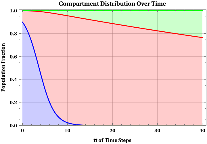
Plotting the differential equation solution for each function on the same plot with regards to the elapsed time intervals. A legend is created to indicate which colored function is which compartment. The second visualization simply fills in the area percentage region each compartment occupies.
In[]:=
Plot{susceptibleSolution[t],infectiousSolution[t],recoveredSolution[t]},{t,0,time},,PlotLegends->{"S (susceptible)","I (infectious)","R (recovered)"}
Out[]=


In[]:=
PlotAccumulate[{susceptibleSolution[t],infectiousSolution[t],recoveredSolution[t]}]//Evaluate,{t,0,time},,Filling->{1->Axis,2->{1},3->{2}},PlotLegends->{"S","S + I","S + I + R"}
Out[]=
SEIR (Susceptible-Exposed-Infectious-Recovered)
SEIR (Susceptible-Exposed-Infectious-Recovered)
Introduction & Overview
Introduction & Overview
Next, we will explore the SEIR model. Using this model introduces an additional compartment, the “exposed”. As the name suggests, this compartment consists of individuals who have been exposed to trachoma disease and infected by it, but are not yet capable of spreading it yet. Trachoma has an incubation period range of 5-12 days, during which the infected individual may not show any signs of symptoms and remains relatively noninfectious. However, once those symptoms develop, they become significantly more infectious.
The implementation code for SEIR is very similar to SIR, the difference being the rates and initial constants needed to account for the exposed compartment.
Defining Initial Constants and Rate Constants
Defining Initial Constants and Rate Constants
The initial exposed compartment is defined as 0, as well as the transmission rate (rate at which people who are susceptible are exposed to the disease) and incubation rate (rate at which people who are exposed become infectious). The other initial values and rates that were defined in the previous section on SIR remain the same. Exposure rate is expressed as (transmissionRate)*I/N so once the transmission rate is set, you automatically have exposure rate.
In[]:=
exposedInitial=0transmissionRate=0.6incubationRate=0.083time=60
Out[]=
0
Out[]=
0.6
Out[]=
0.083
Out[]=
60
Establishing and Solving for the Set of Ordinary Differential Equations
Establishing and Solving for the Set of Ordinary Differential Equations
In[]:=
eqS=sus'[t]==-transmissionRate*inf[t]*sus[t]eqI=inf'[t]==incubationRate*exp[t]-recoveryRate*inf[t]eqR=rec'[t]==recoveryRate*inf[t]
Out[]=
′
sus
New differential equation for the exposed population compartment
Solving for all four differential equations including the one for the exposed compartment
Obtaining the solution for the exposed compartment
Plotting the Function Solutions with Respect to Time
Plotting the Function Solutions with Respect to Time
Plots now include an extra fourth line for the exposed compartment
SIRS (Susceptible-Infectious-Recovered-Susceptible)
SIRS (Susceptible-Infectious-Recovered-Susceptible)
Introduction & Overview
Introduction & Overview
The final infectious disease model that will be explored is the SIRS model. This variation adds another level of complexity to the original SIR Kermack-McKendrick model by adding a variable to the differential equation set of the SIR model that represents the rate recovered individuals lost immunity and return to the susceptible state.
For a bit of context, the species of bacteria that causes trachoma disease is “chlamydia trachomatis”. This bacteria has multiple serotypes of itself (variations of the same specie of bacteria), all of which can induce trachoma within a person’s body. The existence of these serotypes means that a person’s immune response to trachoma disease will only be able to provide partial protection against a specific serotype, but not all of them. Also, factors that increase the likelihood of contracting trachoma disease such as poor sanitation, crowded living conditions, and the presence of fly vectors (e.g. Musca sorbens) and easily lead to reinfection.
Thus, the SIRS infectious disease model is relevant to trachoma disease and will be modelled.
Defining Initial Constants and Rate Constants + Birth & Death
Defining Initial Constants and Rate Constants + Birth & Death
In addition to adding a rate to represent the rate at which individuals lose immunity, we will also implement two other rates to account for the natural birth and death of the population. Initial compartment sizes and recovery rate remain identical to their original definitions above.
Establishing and Solving for the Set of Ordinary Differential Equations
Establishing and Solving for the Set of Ordinary Differential Equations
Adding birth and death rates for the population leads to a lot more complexity!
Solving and obtaining solutions for each population compartment is the same as SIR, the difference lies in what the original differential equations are.
Plotting the Function Solutions with Respect to Time
Plotting the Function Solutions with Respect to Time
Creating the visualization for SIRS is the same for SIR as well.
Modeling Number of Cases Over Time
Modeling Number of Cases Over Time
Data Extraction
Data Extraction
As shown below, we first begin by importing a recent dataset from 2019 detailing the countries and number of cases per 100,000 people each year:
According to the Centers for Disease Control and Prevention (CDC), in Ethiopia, as of 2021, less than 10% of households have access to hygiene and handwashing facilities. Additionally, the country’s poverty level was reported to be 31.4% in 2023. Furthermore, in South Sudan, the poverty rate stands at 79.4%, and only 11% of households have access to basic hygiene and sanitation facilities. Based on the dataset, Ethiopia and South Sudan exhibit some of the highest rates of trachoma globally, making them valuable candidates for simulations that draw attention to the rapid spread of the disease.
Data Cleaning
Data Cleaning
After organizing trachoma case data for all countries from 1990 to 2019, our next step is to define variables that store the number of cases and corresponding years, focusing specifically on Ethiopia and South Sudan given their status as having the highest rates of trachoma worldwide.
We begin by defining the variable ' numCasesEthiopia' and use it to extract the number of cases per 100, 000 people in Ethiopia, organizing the information into a list
Now, we define the variable ‘yearEthiopia’ and extract the corresponding years that the trachoma data for Ethiopia cases ranges from, organizing this information in a list
Now, we must repeat the same steps of extracting and storing the trachoma data for South Sudan. First, we define the variable ‘numCasesSS’ and extract the trachoma data for the number of cases per 100,000 people in South Sudan, once again organizing the data in a list
Lastly, we define the variable ‘yearSS’ and extract the trachoma data for all years the South Sudan data ranges from, organizing the data in a list
Modeling Trachoma Data
Modeling Trachoma Data
Having four variables that contain the data for the number of trachoma cases and corresponding years in Ethiopia and South Sudan, we can now use these variables to generate an interactive graph. This graph will visually represent the relationship between the years and the number of trachoma cases for both countries.
This visualization is valuable as it enables us to observe the differences in the number of trachoma cases between the top two countries with the highest rates. It also illustrates that despite a decline in cases over time due to advancements in healthcare and sanitation facilities, trachoma remains a significant issue. For example, in 2019, the prevalence in Ethiopia was notably higher at 1352.8 cases per 100,000 people compared to South Sudan, which had a prevalence of 341.598 cases per 100,000 people.
This visualization is valuable as it enables us to observe the differences in the number of trachoma cases between the top two countries with the highest rates. It also illustrates that despite a decline in cases over time due to advancements in healthcare and sanitation facilities, trachoma remains a significant issue. For example, in 2019, the prevalence in Ethiopia was notably higher at 1352.8 cases per 100,000 people compared to South Sudan, which had a prevalence of 341.598 cases per 100,000 people.
Displaying the trachoma cases for Ethiopia and South Sudan as a graph over time
Geographical Spread of Trachoma in Ethiopia
Geographical Spread of Trachoma in Ethiopia
Overview of Community Graphs
Overview of Community Graphs
Community graphs serve as useful visuals to illustrate how a disease is predicted to spread in a specified population over time. These graphs help simulate and study disease transmission, utilizing network connections to analyze the movement of infections within specific groups and the broader population.
In community graphs, nodes symbolize individuals or entities within a population, each with unique attributes such as age or health status. The edges, depicted as lines connecting nodes, indicate relationships between individuals, representing how diseases can propagate through physical or social interactions.
In community graphs, nodes symbolize individuals or entities within a population, each with unique attributes such as age or health status. The edges, depicted as lines connecting nodes, indicate relationships between individuals, representing how diseases can propagate through physical or social interactions.
Basic Data
Basic Data
In order to gather basic data of cities and populations in Ethiopia, we first extract a list of all cities in Ethiopia, as displayed below:
Populations
Populations
After displaying the city names in Ethiopia, we can proceed by using a map to create and display a list of these cities with their corresponding populations in Ethiopia
Nearest Cities
Nearest Cities
Afterwards, we can create a function that allows the user to generate the five nearest cities to a specified city, defined as variable ‘exampleCityName’. For this example, we define exampleCityName as Bahir Dar, the capital of the Amhara region of Ethiopia which is proven to have the highest rate of trachoma in the country:
In order to make sure that the specified city is not included in this list, we delete the specified city- targetCity- from the nearestCities list and print the updated nearest cities once again as a list:
Spread Level
Spread Level
As of 2022, in the Amhara region of Ethiopia, the trachoma infection rate is approximately 6%, indicating that in areas affected by trachoma, the disease infects around 6% of the population annually.
First, we can extract the population of Bahir Dar using the cityPopulationList defined earlier:
Now, we can use this population of Bahir Dar to calculate the number of individuals expected to be affected by trachoma each year. Subsequently, we can determine the critical number of years it will take for a significant portion of the population in Bahir Dar to become infected.
According to the calculation above, we can assume that trachoma will infect around 14,598 people each year if it maintains a population of around 243,300 people, and it will take around 16.667 years for Bahir Dar to reach a critical number of people infected with trachoma.
Because trachoma will also infect the five neighboring cities found earlier at the same infection rate of 6%, we can repeat the same steps for the neighboring cities to calculate how many years it takes for each city to become critically infected:
Adet:
Werota:
Motta:
Addis Zemen:
Debre Tabor:
Trachoma Community Graphs
Trachoma Community Graphs
Setting up the Community Graph
Setting up the Community Graph
Continuing the example of Bahir Dar, we can first create a community graph where we connect Bahir Dar to its five nearest cities generated earlier:
Since the starting location in this simulation is in Bahir Dar, the following code allows us to color the Bahir Dar node red, indicating that it is infected:
Then, we can proceed by creating a function below that allows us to specify the city that we want to be the starting point of the infection. Below, we listed Bahir Dar as the starting point; however, this point can easily be changed by the user to another nearby city by utilizing the makeGraph function created:
Below, we are constructing community graphs to show when cities get infected in 10-year intervals. The order of infection and timing are based on the time it took for a country to reach its critical infection number, calculated with the trachoma infection rate (1%) and city populations. Each graph represents a different time interval, with the nodes gradually colored in red to depict city infections over time.
Finally, we can animate the coded community graphs from above to visually depict the rapid spread of trachoma among neighboring cities.
Future Work
Future Work
In the future, we aim to simplify the process of creating community graphs by automating the entry of infection data for different cities. Instead of manually inputting and extracting data for each city, such as Bahir Dar, developing a function that can smoothly execute these steps for any city specified by the user would be a more efficient approach. By doing so, we are interested in improving efficiency over repetitive manual inputs when generating the community graph animation. Furthermore, we hope to delve deeper in how the SIR/SEIR models vary for trachoma among different regions of the world, each with different levels of trachoma infection rates and portions of the population currently infected, as well as how these models compare to SIR models for other eye diseases.
Conclusion
Conclusion
Our project on modeling trachoma disease using variations of the SIR model, unique sets of ordinary differential equations, and community graph networks has been successful. Through the application of complex mathematical frameworks and visual representations, we accurately modeled trachoma and presented our results. Additionally, we deepened our understanding of infectious disease dynamics as a whole and the patterns by which diseases can be transmitted. The success in modeling trachoma disease demonstrates the effectiveness of SIR model variations and graph networks. These tools enable researchers to gain valuable insights during future disease outbreaks. Health officials can also utilize these tools to predict the behavior of a disease in response to intervention strategies aimed at reducing disease transmission, such as the practice of quarantining during the COVID-19 pandemic. Overall, the tools explored in this project are extremely relevant and useful in the context of the real world.
References
References
1
.“Trachoma.” Centers for Disease Control and Prevention, Centers for Disease Control and Prevention, 15 June 2022, www.cdc.gov/hygiene/disease/trachoma.html. Accessed 10 Oct. 2023.
2
.“The Sir Model for Spread of Disease - the Differential Equation Model.” The SIR Model for Spread of Disease - The Differential Equation Model | Mathematical Association of America, maa.org/press/periodicals/loci/joma/the-sir-model-for-spread-of-disease-the-differential-equation-model. Accessed 13
3
.Nov. 2023.
4
.“Trachoma Prevalence Rate.” Our World in Data, ourworldindata.org/grapher/trachoma-prevalence-age-standardized-ihme. Accessed 15 Nov. 2023.
5
.6
.“What Is Trachoma?” Sightsavers, 6 Nov. 2023, www.sightsavers.org/protecting-sight/ntds/what-is-trachoma/.
7
.Wanza, Serah N. “What Is the Bazaar Fly?” WorldAtlas, WorldAtlas, 5 Jan. 2018, www.worldatlas.com/articles/what-is-the-bazaar-fly.html.
8
.“Kermack-McKendrick Model.” From Wolfram MathWorld, mathworld.wolfram.com/Kermack-McKendrickModel.html. Accessed 28 Nov. 2023.
9
.Genet, Almaw, et al. “Prevalence of Active Trachoma and Its Associated Factors among 1–9 Years of Age Children from Model and Non-Model Kebeles in Dangila District, Northwest Ethiopia.” PLOS ONE, Public Library of Science, journals.plos.org/plosone/article?id=10.1371%2Fjournal.pone.0268441.
10
.Accessed 29 Nov. 2023.
11
.Pinsent, Amy, and Manoj Gambhir. “Improving Our Forecasts for Trachoma Elimination: What Else Do We Need to Know?” PLoS Neglected Tropical Diseases, U.S. National Library of Medicine, 9 Feb. 2017, www.ncbi.nlm.nih.gov/pmc/articles/PMC5321453/.
12
.“Trachoma.” Mayo Clinic, Mayo Foundation for Medical Education and Research, 21 Oct. 2020, www.mayoclinic.org/diseases-conditions/trachoma/symptoms-causes/syc-20378505.
13
.Yongli Cai a, et al. “A Stochastic SIRS Epidemic Model with Infectious Force under Intervention Strategies.” Journal of Differential Equations, Academic Press, 8 Sept. 2015, www.sciencedirect.com/science/article/pii/S0022039615004271#fm0010.
“The SEIR Model of Infectious Diseases ¶.” 09_SEIR_model, web.pdx.edu/~gjay/teaching/mth271_2020/html/09_SEIR_model.html. Accessed 17 Dec. 2023.
“The SEIR Model of Infectious Diseases ¶.” 09_SEIR_model, web.pdx.edu/~gjay/teaching/mth271_2020/html/09_SEIR_model.html. Accessed 17 Dec. 2023.
CITE THIS NOTEBOOK
CITE THIS NOTEBOOK
Utilizing SIR Model Variations (Ordinary Differential Equations) and Community Graph Network
by Wolfram Emerging Leaders Program
Wolfram Community, STAFF PICKS, January 2, 2024
https://community.wolfram.com/groups/-/m/t/3094917
by Wolfram Emerging Leaders Program
Wolfram Community, STAFF PICKS, January 2, 2024
https://community.wolfram.com/groups/-/m/t/3094917