Generating Images using Sinusoidal Lines with various frequencies and line widths and connecting lines Allen Gary CSPAR/UAH 10 September 2026 Used Bezier curves to connect the sine curves and semi-circle connections between rows
Generating Images using Sinusoidal Lines with various frequencies and line widths and connecting lines Allen Gary CSPAR/UAH 10 September 2026 Used Bezier curves to connect the sine curves and semi-circle connections between rows
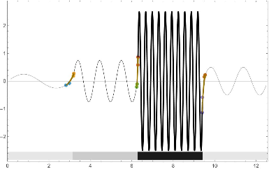

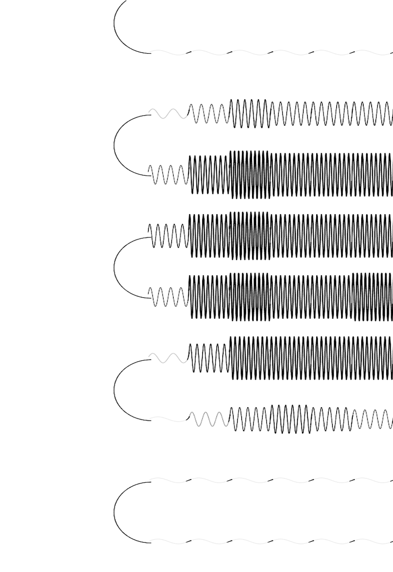
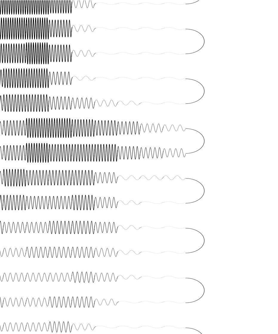
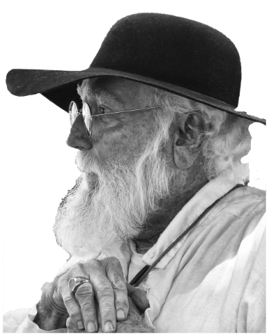
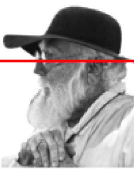
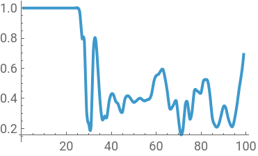
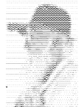
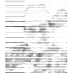
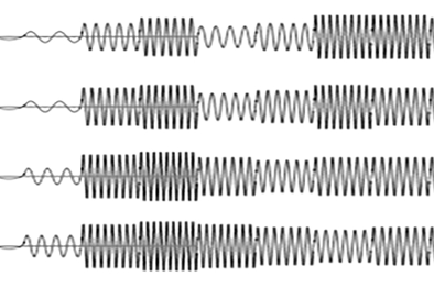
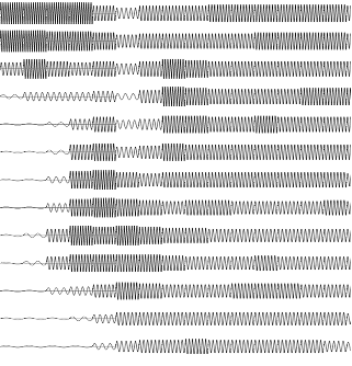
Introduction: This program, “Generating Images Using Sinusoidal Lines with Variable Frequencies and Line Widths,” transforms a black-and-white image into a continuous artistic rendering composed of sinusoidal curves. Each row of pixels in the original image is analyzed and converted into a single, continuous sine wave whose frequency, amplitude, and line thickness vary according to the pixel values. Bezier curves connect the sine curvesBy modulating these parameters, the program recreates the tonal structure and visual details of the source image using oscillating lines rather than discrete pixels. The resulting artwork combines mathematical visualization with artistic expression, producing images that resemble hand-drawn line art while retaining the recognizable features of the original photograph. This approach demonstrates how mathematical functions can be used as creative tools for image generation and transformation. The work of artist Tyler Foust, known for his intricate continuous-line portraits, served as partial inspiration for the development of this program.ReferencesWolfram Community: Generating Images Using Sinusoidal Lineshttps://community.wolfram.com/groups/-/m/t/3775425?p_p_auth=szILJul8My Modern Met: Tyler Foust’s One-Line Drawing Portraitshttps://mymodernmet.com/tyler-foust-one-line-drawing-portraits/?utm_source=Pinterest&utm_medium=organic The pixels of under the red line Program Result of Image made of Sine Curves Enlarged area of noise and eye

Load Image
Load Image
In[]:=
ClearAll["Global`*"]
In[]:=
SetOptions[$FrontEnd,"DynamicEvaluationTimeout"->600]
In[]:=
imageFile="C:\\Users\\gag00\\Line Portraits\\portrait50x63.jpg";(*inputimagefilename500x626@JuliaGary*)
img=ColorConvert[Import[imageFile],"Grayscale"];
In[]:=
pixels=ImageData[img];
In[]:=
rows=ImageDimensions[img][[1]];columns=ImageDimensions[img][[2]];{rows,columns}
Out[]=
{50,63}
Rasterize image to smaller size
In[]:=
rastersize=1;
In[]:=
rasterized=Table[Mean[Flatten[pixels[[i;;i+rastersize,j;;j+rastersize]]]],{i,1,columns-rastersize,rastersize},{j,1,rows-rastersize,rastersize}];
In[]:=
dim=Dimensions[rasterized];rows=dim[[1]];cols=dim[[2]];{rows,cols}
Out[]=
{62,49}
In[]:=
rasterized[[49,1]]=0
Out[]=
0
Image[rasterized];
In[]:=
sinecurvethickness=LinearModelFit[{{1.,.00005},{3.,.00010},{10.,.00050},{2.,.00007},{5.,.00030}},x,x];
In[]:=
TransitionCurve[pts_,w1_,w2_,j_]:=Module[{xycurve,ts,points,normals,widths},bez=BezierFunction[pts];du=0.1;us=Range[0,1-du,du];segments=Table[{Thickness[sinecurvethickness[amp[[j]]]],Line[{bez[u],bez[u+du]}]},{u,us}];segments](*Beziercurvesfortransitionsgiven2ptsforeachsinecurve*);
In[]:=
Evaluative
In[]:=
xsize=49;(*xpixelwideyhorizontallines*)ysize=62;xn=3(*linelocationdowntheimage*);
In[]:=
makeGraphic[frequency_]:=Module{plot},xn=frequency;offset=Table[(i-1)*π,{i,xsize}](*offsetalongrowsforeachsinecurve*);ydata:=rasterized[[xn,;;]](*forgivenrowthegraylevels*);xdata=Range[Length[ydata]](*;f=Interpolation[ydata];*);Clip[(10-Round[ydata*10]+1),{1,10}];amp=Clip[(10-Round[ydata*10]+1),{1,10}];w=ConstantArray[1.,xsize];w[[1;;8]]:={0.020,0.020,0.02,0.03,0.04,-0.02,0.02,0.01};xycurve[x_,nthcurve_]:={x+offset[[nthcurve]],5.(amp[[nthcurve]]/20.)Sin[2.xamp[[nthcurve]]]};Off[Solve::ifun];ydelta[amp_]:=-0.1*amp;y[x_,ampp_]:=5.(ampp/20.)Sin[2.xampp];sol=Solve[5.(ampp/20.)Sin[2.xampp]-ys==0,x];PositionAmpxyXY=ConstantArray[1.,{2,10,5}](*left/rightampx1,y1,x2,y2*);xlocation[ys_,ampp_]=x/.sol;xxend[ys_,amp_]:=Pi+xlocation[ys,amp][[1]];xx[ys_,amp_]:=-xlocation[ys,amp][[1]];asel=2;xx[ys_,amp_]:=Pi+xlocation[ys,amp][[1]];Do[xp=xx[ydelta[amp],amp];yp=y[xp,amp];xp2=xx[ydelta[amp/2.],amp];yp2=y[xp2,amp];PositionAmpxyXY[[2,amp]]={xp,yp,xp2,yp2},{amp,1,10}];asel=1;xx[ys_,amp_]:=-xlocation[ys,amp][[1]];Do[xp=xx[ydelta[amp],amp];yp=y[xp,amp];{xp,yp,amp};xp2=xx[ydelta[amp/2.],amp];yp2=y[xp2,amp];PositionAmpxyXY[[1,amp]]={xp,yp,xp2,yp2},{amp,1,10}];BpR2[i_]:=PositionAmpxyXY[[2,i,3;;4]];BpL2[i_]:=PositionAmpxyXY[[1,i,1;;2]];BpR1[i_]:=PositionAmpxyXY[[2,i,1;;2]];BpL1[i_]:=PositionAmpxyXY[[1,i,3;;4]];points=Table[{BpL1[i],BpL2[i],BpR1[i],BpR2[i]},{i,1,10}];lowvalue=-4.85;highvalue=-2.55;plot=Show
Table
[
ParametricPlot[
xycurve[t,j],
{t,2Pi(1./amp[[j]])/40.,Pi-2Pi(1./amp[[j]])/40.},
PlotStyle->Directive[Black,Thickness[sinecurvethickness[amp[[j]]]]],Frame->False
],
{j,1,xsize}
]
,
Graphics[Table[
Black,TransitionCurve[Flatten[{points[[amp[[j]]]][[3;;
4]]+Threaded[{(j-1)Pi,0}],points[[amp[[j+1]]]][[1;;2]]+Threaded[{(j)Pi,0}]},1],
w[[1]],w[[2]],j],{j,1,xsize-1}]
,Frame->False]
,
PlotRange->{{0,49π},{-2.9,2.9}},PlotRangeClippingTrue,PlotRangePadding->None,ImageMargins->0,Axes->False,Frame->False,AspectRatio->130,FrameStyleDirective[White,12];plotEnd of Program