“I can’t understand anything in general unless I’m carrying along in my mind a specific example and watching it go. Some people [think] I’m following the steps mathematically, but that’s not what I’m doing.” — R. P. Feynman
Abstract
Abstract
This tutorial offers a bridge between the abstract mathematics of differentiable manifolds and computational practice. Computational practice means writing software in terms of matrices and vectors containing real and complex numbers. We offer elementary examples fully explained and illustrated at length.
Nowadays, some understanding of differential geometry and topology is increasingly necessary even if your only objective is to do calculations, not to do proofs. That’s because differential geometry and topology have crept from mathematics and physics into engineering. In simulation, robotics, and computer games, they support much better numerical performance than do older approaches.[19][20] Philosophically, it seems that differentiable manifolds, in 3, 4, 8, and more dimensions, rule all the natural World, all the way from quarks through robots to black holes and superclusters of galaxies. Differential geometry offers one set of tools for all these domains in place of many sets of incompatible tools, one for each domain.
Contemporary books and papers on applications of differential geometry and topology can be challenging. Many are written in highly abstract mathematical style (definitions and proofs without examples), with more generality than needed for applications (unphysical topologies), and with unfamiliar notation. If you didn’t learn fiber bundles, exterior calculus, and Lie theory in school and you want to catch up fast, this tutorial might be interesting to you. You’ll be equipped to read papers without choking on things you’ve never heard of, to get through to the juicy bits where we learn from the heavy math how to do calculations.
Looking forward, I have some notebooks in the works on integrating equations of motion of mechanical systems on Lie groups. The Lie groups needed for simulation and control are differentiable manifolds, abstract curved spaces analyzed through differential geometry and topology.
Prerequisites
Prerequisites
We assume linear algebra and multivariable calculus: typical undergraduate applied mathematics for engineering and science. We do not assume topology, point-set topology, real analysis, tensors, exterior algebra and calculus, differential forms, generalized Stokes’ theorem, Lie groups, Lie algebras, or Hodge theory. We do not even assume basic concepts of pure mathematics, like equivalence class, set theory, bijection, surjection, and partial function.
The following terms should immediately bring to mind a concrete realization and a calculational procedure, i.e., we assume you know how to write software with them: matrix, inverse, transpose, determinant, column vector, row vector, divergence, gradient, curl, Jacobian, Hessian. We also assume you know that column and row vectors are punned as flat lists in Mathematica.
Cheat Sheet
Cheat Sheet
The following table summarizes chapter 4 of Reference [14]. To keep it small, it is not self-contained, but rather presented in very roughly the order of this tutorial to help you jump to various parts, also as a reference to return to. Many items might not be understandable without forward reading. Reference [14] is authoritative for details and in the case of errors in the table and in the rest of this document. The red highlighted item is a particularly obtuse bit of notation, and we explain it at length in the body of the tutorial.
NOTION | NOTATION | DEFINITION | REMARKS |
Manifold | M N | abstractcollectionofabstractpoints | adddifferentiablestructure |
CoordinateChart | (U,φ) | U⊂M,Uopenφ:U↔φ(U)⊂ n | φ(m)={ 1 x 2 x n x |
OpenSet | U U | primitivefromtopology | detailedknowledgenotneeded |
CompatibleCharts | (U,φ),( ′ U ′ φ | ′ φ -1 φ ′ U ∞ C ′ U ′ φ ′ U | |
DifferentiableManifold | Every m∈M | M | |
DifferentiableStructure | Maximalatlas | Collectionofallcompatiblecharts | |
Neighborhood | -1 φ n | Hausdorfftopology: m≠m' | |
Equivalentcurves | c 1 c 2 ′ (φ◦ c 1 ′ (φ◦ c 2 | c 1 c 2 | forsomechart φ |
TangentVector | v(m) | Equivalenceclassofcurves | |
EquivalenceClass | [c(t)] | Allcurveswithsamevalueandderivativesthroughsomechartφatt=0 | |
Tangentelsewhereonacurve | ∀c(t),def ′ c dc dt t=0 | ′ c | t=0 | finitedistance s c(t) |
TangentSpace | T m | Spaceofalltangentvectorsat m∈M | THEOREM: T m |
ComponentsofaVector | i v d dt i (φ◦c) | t=0 | Superscriptrunsoverthedimensions | Eachcomponentisarealnumber |
TangentBundle | TM= T m m∈M | Includeslocalcoordinatesandcomponentsofvectors | dimensionis 2n |
NaturalProjection | τ M -1 τ M T m | Returnsattachmentpointofavector | -1 τ M TM m |
Differentiable,Derivative | With f:MN T m T m T f(m) | T m T m T m dc dt t=0 d dt t=0 | M N |
Diffeomorphism | f:MN | Bijective,differentiable,&diff'bleinverse | donut&coffeecuparediffeomorphic |
Motivating Example
Motivating Example
Get Your Kicks on Route 55
Get Your Kicks on Route 55
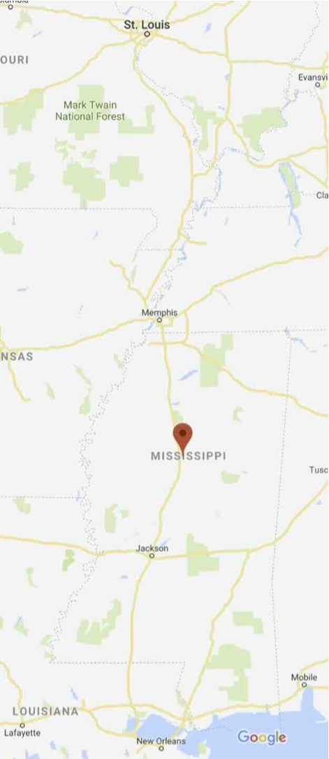
Let , a manifold, be a set of abstract points representing a part of the surface of the Earth between St. Louis in the North and New Orleans in the South, and wide enough for the Mississippi River. We call it a manifold because it’s many-folded, that is, curved. Though this one doesn’t have many folds, more general cases do.
M
This manifold, however, is sufficiently curved to be interesting and illustrative. To start, is just a set of points on the globe. There is obvious organization of the points. It is obvious to say that "Memphis is between St. Louis and New Orleans" and "Interstate 55 roughly follows The River." But we don't yet know how to be precise in those statements because of the curvature. We know Euclidean geometry, Cartesian analytical geometry, and trigonometry we learned in school, and we know they don’t work on curved surfaces. We can’t calculate the distance from St. Louis to New Orleans simply by subtracting their latitude-longitude coordinates. The math we know only works on flat surfaces. Can we relate the math we know to this globe? That’s the topic of differentiable manifolds in a nutshell: relating sets of points on curved manifolds to flat, Euclidean hyperplanes where we know how to calculate. Sometimes, the curved manifolds like the globe have two dimensions. Sometimes, they have many more. The SU(3) group of quantum chromodynamics is a manifold of eight real dimensions (https://en.wikipedia.org/wiki/Special_unitary_group).
M
Out[]=
Definition: Parameterized Curve
Definition: Parameterized Curve
Imagine a collection of parameterized curves that map real numbers (parameters) to points in the manifold, the globe in our example. Denote one member of that collection as . is a function. The value of that function, , given a real number , is a point in the manifold. As , a real number, advances, names one point on the Earth’s surface, then another point nearby, then another even further, and so on.
c
c
c(t)
t
m∈M
t
c(t)
How do we “name” points in the manifold and how we decide what “nearby” means? Don’t say “latitude and longitude!” just yet, because that’s a particular numerical scheme, a chart, and we’re not there yet. There are lots of other ways to name points on the Earth’s surface.
Definition: Point
Definition: Point
What’s a point? It’s smaller than a ten-foot square. It’s smaller than an inch. It’s smaller than an atom. It’s smaller than an atomic nucleus.
Physics hints that we can’t measure anything smaller than the Planck length, about cm, so that will do. That’s really small, by the way: a hundred million trillion () times smaller than an atomic nucleus, which is about cm across. If we can uniquely name any little Planck square, cm on a side, anywhere on the globe, could anyone ask for anything more in the real world?
-33
10
20
10
-13
10
-33
10
Mathematicians, of course, reason outside the real world with uncountable infinities of infinitesimally small points. Such reasoning is necessary for a rigorously logical understanding of calculus, but we don't go that far. We're trying to stay concrete. See ref [15] for a beautiful account of calculus from a rigorously logical point of view. The abstract notation we’re explaining in this tutorial assumes you have heard of that point of view, which is artificially and ironically called real analysis, based on point-set topology. You don’t have to be proficient in those topics to do calculations.
What3Words: Unique Names for Ten-Foot Squares
What3Words: Unique Names for Ten-Foot Squares
The web site "What3Words.com" gives a unique name to every ten-foot square on the surface of the Earth (it might not work very close to the North and South Poles).
Pick some point on the surface. We showed above that, for practical purposes, a point is a Planck square. Pick a specific Planck-square in a specific nucleus of a specific atom in a specific USGS geodetic marker in Winona, Mississippi, the seat of Montgomery County. "What3Words" has a unique name for the ten-foot square that encloses our point. That name is "jokers.priced.pursuit" (https://map.what3words.com/jokers.priced.pursuit).
The important point is that these three-word string-names contain no metrical information. Given two string-names, it’s impossible to tell whether the corresponding ten-foot squares are adjacent or ten thousand miles apart. From a user’s point of view, the names are randomly chosen.
What21Words: Unique Names for Planck Squares
What21Words: Unique Names for Planck Squares
Definition: Manifold
Definition: Manifold
Aside: Do-It-Yourself Naming
Aside: Do-It-Yourself Naming
If you are not interested in how to name points and squares with strings of words, nor in my guesses about how “What3Words” works, skip this section.
It’s interesting to figure out how “What3Words” might work. This is my guess.
What4Words: Using My Own Dictionary
What4Words: Using My Own Dictionary
Names for Planck Squares
Names for Planck Squares
We want to uniquely name every Planck square on Earth. How many of my words would we need?
We have a practical scheme for naming every Planck square on Earth: every point that is a hundred million trillion times smaller than an atomic nucleus named with just twenty-one words in a string.
It would not be secure. A dedicated hacker could discover our systematic scheme and then clone our site. How “What3Words" protects their intellectual property is anyone's guess, but if I were they, I might just use a random distribution and a database. It's just barely practical to have a database of 56 trillion items (e.g., InnoDB can do it). Lots of interesting crypto tricks like zero-knowledge proofs are conceivable, too, but let’s get back on track with manifolds.
We’re using the same name for the ten-foot square from “What3Words” and for our specific Planck square in our specific nucleus or our specific atom of our specific geodetic marker in Winona, MS, but we won’t get confused.
Differentiable
Differentiable
from a point in New Orleans, 600 miles away, say "joins.slides.predict?"
Even if two points are really close, say the lamppost "bottle.ruled.varieties" in St. Louis
and the next lamppost at "heavy.beyond.speeds,"
we don't know how to "subtract" them. We can subtract angles or vectors, but not points.
Definition: Chart
Definition: Chart
We need a chart, a way to convert points in the manifold to numerical things like angles or vectors. We’re only going to work with a trivial chart to keep this example simple and easy, but take a look at Wikipedia’s collection of map projections https://en.wikipedia.org/wiki/List_of_map_projections. Coming up with charts is difficult and is, in fact, a principal problem for mapmakers and manifold theorists. Many of these map projections were specially constructed in earlier times when people calculated distances, headings, and areas by hand or even in their heads. Various map projections are specialized for distances, angular headings, or areas, but can’t support all three, or even more than one, efficiently. A human navigator may need several charts to get the job done. Many charts are set up for physical measurements on flat paper with protractor, ruler, and compass. We still use those charts in computers, just with virtual protractors, rulers, and compasses.
Distances: Coordinate and Metrical Distances
Distances: Coordinate and Metrical Distances
The web API (not necessarily the GUI) of “What3Words” implements a chart: you give it a three-word name and it gives you back a latitude and longitude. Latitudes and longitudes won’t yield distances directly by subtraction, but we can compute purely formal sums and differences, called coordinate distances. We’ll construct a slightly complicated function below that produces metrical distances from lats and lons — actual feet and miles on the ground that you’d get from an odometer. We won’t get into complicated charts like Wikipedia’s map projections. The purpose of this tutorial is to help you appreciate manifolds from simplified examples, not to get you into all the details.
Definition: Open Sets (Trouble at the Poles)
Definition: Open Sets (Trouble at the Poles)
Many charts of the Earth have trouble near the North and South Poles, but people don't ordinarily go to either place, so cartographers often park troublesome bits at the poles. “What3Words" goes way up in latitude, but I haven't found the North Pole, yet, because their display-maps don't show anything up there and I can't see what I’m doing. The South Pole seems to be at "greenhouses.recommitting.multiplexes" because the maps go crazy there and the web app doesn't behave well. We shouldn't play around where we know someone else's web app chokes up; that's a denial-of-service attack. So I gave up at the first sign of trouble, but there was trouble. Maybe it’s fixed, now.
In manifolds, we work with open sets, a purely formal, logical notion in topology. Open sets make calculus work by excluding troublesome bits. Our main goal, after all, is to make calculus work, so we mention open sets frequently in the statements and proofs of theorems. You don’t need to know topology to get through this tutorial, but you must resort to the formalities to strike out on your own.
Intuitions about open sets are notoriously misleading. Some sets can be both open and closed, and some sets can be neither open nor closed. It took 300 years to make calculus rigorously logical, after all, even though it was working well for physics and engineering from the days when Newton and Leibniz invented it. In fact, there is evidence that Archimedes, almost 2000 years prior, had the inklings of calculus (https://www.amazon.com/Archimedes-Codex-Revealing-Antiquitys-Scientist/dp/030681580X). See References [15] and [18] if you’re driven to know the topology behind calculus.
For applications in physics and engineering, the example of "trouble at the poles" is the intuition needed to understand an open set. You can go near a pole, and maybe inch a little nearer, and a littler nearer, but eventually you'll reach the limits of some practical computation and that will be the end of your session. You might as well have hit the excluded point dead-on.
Definition: Dimension
Definition: Dimension
Any chart on the Earth must let us convert three-word names or features like lampposts to pairs of numbers. We can't do with fewer than two numbers per point, and three wouldn't help. We’re near the Mississippi River and we’re not paragliding or mining. The Earth manifold represented by any chart is two-dimensional, exactly two-dimensional. Likewise, any chart of the Lie Group SU(3) must have exactly eight dimensions.
Definition: Derivative of a Curve Through a Chart
Definition: Derivative of a Curve Through a Chart
At that latitude, one increment-in-last-place of longitude, using easy spherical trigonometry, is about
Definition: Function Composition
Definition: Function Composition
What Does “Nearby” Mean?
What Does “Nearby” Mean?
A First Curve
A First Curve
A Second Curve
A Second Curve
Definition: Tangent Vector
Definition: Tangent Vector
That angle is a metrical property that pertains only to that one point, and that's why it's called tangent: the two derivative sets inhabit the same flat 2-space, where all our school math like dot product works. But the flat 2-space is glued to exactly one point of the manifold. The curved surface of the manifold falls away from the tangent plane on all sides, making metrical calculations difficult. Dot products of 2-vectors only work in flat 2-spaces with the basic orthogonal coordinate system and when the vectors are rooted at the same point.
Aside: Only Direction Matters?
Aside: Only Direction Matters?
Rewrite Equation 4:
Any Old Chart Will Do
Any Old Chart Will Do
Metric Tensor: Restoring the Dot Product
Metric Tensor: Restoring the Dot Product
In fact, the dot product should not depend at all on the choice of chart. It should work not only in sheared coordinates, but in curvilinear coordinates of any kind, so long as the chart doesn’t have any singular structures, like poles, caustics, creases, etc., that is, any structure where a point in the manifold does not have unambiguous coordinates. The transformation from the basic chart to the sheared chart doesn’t have any such bad features so long as we don’t completely collapse it to a line. That means that the transformation from the basic chart to the sheared chart is a function with an inverse. Later, we’ll add the restriction that all derivatives of the transformation exist and and are well-behaved (in open sets) both to and from the basic chart. In this example, the dot product must take into account the shearing.
The general form we are looking for is
Our present job, though, is to find the matrix representation of the metric tensor for any reasonably sheared chart. The ShearTransformation must contain the information we need for the matrix. Our job is to fish that information out.
The machinations above were designed to produce a pleasing demonstration, with the origin displaced from the lower-left corner. Those machinations are now getting in the way of analysis (they’re forcing us into affine transformations, which are non-linear in the coordinates, and we don’t want them now). Let’s get rid of the displacement. The highlighted lines reveal the metric tensor, and we’ll explain it after the demonstration.
Take a deep breath. Let’s explain what we see above. We’ll have to relate it to the code.
First are the two vectors with some whimsically chosen components in the basic, unsheared, orthogonal, Cartesian coordinate frame.
These are just lists of numbers in the code. Mathematically, they are column vectors: lists of lists amounting to 2 rows and 1 column. They should be
Mathematica finesses this point (irritatingly), so we shall also, for now. But it becomes critical for understanding the mathematics later, when we introduce co-vectors as row vectors in the co-tangent space. In the highlighted line of the demonstration, we emphasize the mathematical point by showing an explicit transpose operation on t20$. This transpose does nothing on a flat list, Mathematica’s cringeworthy pun for both a column vector and for a row co-vector. Python does it too, so this pun has leaked everywhere in the Industry, and it gets in the way later.
Next is the shearing-transform function. When we apply that function to the constant coordinate-grid lines, we get Line objects that follow the sheared coordinate axes, which have the same constant values in the sheared coordinates as in the orthogonal coordinates, but are mapped back to Mathematica’s orthogonal screen coordinates. The numbers returned from GeometricTransformation[grid0$, ShearingTransform[...]] are in orthogonal coordinates for plotting, so we deduce that the shearing transform converts sheared coordinates to orthogonal coordinates.
The inverse shearing transform converts orthogonal coordinates to sheared coordinates. The vectors have constant components in the orthogonal coordinate. To get the sheared coordinates of the vectors, apply the inverse shearing transform.
It should now be obvious that the shear-independent dot product is
and that the matrix representation of the metric tensor in the sheared coordinates is
Those tensor components are displayed in the demonstration and they depend on an actual, non-constant shear. Because the dot product in Equation 7 is independent of the particular shear, we deduce that the metric tensor itself, not its matrix representation, must be independent of the shear if the vectors themselves, not their lists of components, are independent of the shear. We go one step further and declare that if the vectors are geometrical entities independent of coordinate system, the metric tensor itself must be a geometrical entity independent of coordinate system. We will find out later that it is a bilinear transformation, and we can regard that as a geometrical object, though not directly visualizable.
Back to the Curves
Back to the Curves
We have one uncountably infinite collection of curves, all with the same 2-vector derivatives as one another through some chart, and another uncountably infinite collection of curves, all with the same 2-vector derivatives as one another through the same chart, but different — not infinitesimally! — from the derivatives in the first collection. We can calculate the angles between any such pair of curves chosen any way we like without considering details of the curves and certainly without considering the charts. So really, the sets of curves act just like vectors, so we just call them that. That's an honest achievement.
Definitions: Equivalence, Atlas, Partition
Definitions: Equivalence, Atlas, Partition
The general concept of a set of things that have something in common is an equivalence class. An equivalence class comprises all things that are equivalent, according to some specific definition of equivalence, and excludes all things that are not equivalent to any member of the class. For our purposes, the word “class” is a synonym for “set,” but there are technical differences concerning logical paradoxes in the theory of sets, deep waters we need not wade in here.
Metrical Distances: Geodesics
Metrical Distances: Geodesics
We’ve got angles and dot products down; let’s measure non-infinitesimal metrical distances. We want metrical distances that are the shortest possible. The shortest distance between any two points on any manifold is the geodesic distance, and the curve (set of points in the manifold) with the shortest integrated distance is the geodesic between those two points. It’s sensible to say the geodesic curve because geodesics are unique, at least up to some technicalities. Geodesic curves are computed through charts by solving certain differential equations.
On the spherical Earth, geodesics are great circles. Other manifolds in common use for the Earth include the ellipsoidal WGS84 and lumpy spherical harmonics. Geodesics on these manifolds follow the ellipses and lumps. They are not circles and they are much more complicated to express. But they harbor no new concepts, so won't help with the purpose of this tutorial, which is to present a simplified example that any of us, including Richard Feynman, could play along mentally.
Let’s see how it does between our favorite points in St. Louis and New Orleans. The API (not the GUI) at “What3Words” gives us lat-lons for our two points:
You can check this on-line at many sites, like http://www.csgnetwork.com/gpsdistcalc.html; it’s good to at least three digits.
Leaving the Real World: Abstract Theory
Leaving the Real World: Abstract Theory
Definition: Tangent Space
Definition: Tangent Space
Tangent Space: Independent of Chart
Tangent Space: Independent of Chart
Tangent Spaces are Vector Spaces
Tangent Spaces are Vector Spaces
A vector space is an abstraction of ordinary intuition on Euclidean vectors as tuples of numbers. The abstraction picks out just those features of ordinary vectors that suffice for linear algebra to work. We want the elements of tangent spaces — equivalence classes of curves — to act just like vectors, so we can apply the entire machinery of linear algebra on them. That’s why this section is important.
What does it mean for equivalence classes of curves to act just like vectors? It means you can add equivalence classes of curves and multiply equivalence classes of curves by scalars. We’ll need artificial definitions of “add” and “multiply.” “Adding” equivalence classes of curves is not set union: it's a special operation defined below.
Begin with ordinary vectors: “ordered tuples of numbers that (1) can be added element-wise to yield more vectors and (2) can be multiplied by numerical scale factors (scalars).” Abstract away four things: the objects being added, the addition operation itself, the type of the scalars, and the multiplication operation between scalars and vectors:
1
.Replace “ordered tuples of real numbers” with abstract undefined objects.
In our case, the abstract undefined objects will be equivalence classes of curves.
2
.Replace "addition" with an artificial definition of "addition." We don't need the concept of "element-wise."
However, we want the artificial definition of addition to act like ordinary vector addition, meaning four things:
Those are four of the eight abstract axioms of a vector space that tangent vectors must satisfy for tangent spaces to be vector spaces.
To summarize, we define addition as follows (there is a lot of stacked notation, here):
3
.replace numerical scalars with (different) abstract objects that only need to be member of some field.
A field, in turn, is an abstraction of the scalars. The axioms for a field are listed here: http://mathworld.wolfram.com/Field.html.
In our case, we stick with real numbers for scalars. The reals are a field. So are the complex numbers, so all this stuff works in quantum theory.
Vector-space axioms are listed at Wolfram MathWorld (http://mathworld.wolfram.com/VectorSpace.html).
A vector space is not the same thing as an abstract vector space (http://mathworld.wolfram.com/AbstractVectorSpace.html); this is a case where we cannot use the word "abstract" loosely.
If that isn’t enough abstraction for you, look into modules (http://mathworld.wolfram.com/Module.html). We won’t need these for our manifolds, but we mention them again when we come to linear maps, which are defined by certain axioms on modules. All vector spaces are modules, so we won’t get lost. But some modules are not vector spaces, and such things show up in applications, not just in pure mathematics. String theory and other exotic, speculative physics need these abstractions.
Type Notation
Type Notation
Consider the following expression:
There is much more to the distinction of types and sets. See https://cs.stackexchange.com/questions/91330/what-exactly-is-the-semantic-difference-between-set-and-type for instance. But the intuition above is enough for us.
Definition: Components of Tangent Vectors
Definition: Components of Tangent Vectors
This is the connection between the modern, coordinate-free notation and the traditional, 19-century notation that Einstein and everyone else used and is documented in Reference [17], the book from which I learned this entire theory. The modern notation literally abstracts out the charts (by a literal definition of the verb abstract that we won’t get into). In the old notation, we can't even talk about points and vectors, let alone more advanced things like tensors and differential forms, without charts and chart-to-chart transformations and the superscripts and subscripts coming with them. The old notation is more cumbersome, but more explicit. The choice of which to use is a trade-off, at least until we get to writing computer programs. Academics have, long since, made the decision for us. We can't read contemporary papers without understanding the modern notation, but we can't write computer programs without translating it, through charts, into the old notation. That's what this tutorial is all about.
Definition: Derivative of a Curve
Definition: Derivative of a Curve
Notation: Lambda Expressions, Anonymous Functions,
Closures, Parameters, Dummy Variables,
Arguments, Function Bodies, Free Variables
Notation: Lambda Expressions, Anonymous Functions,
Closures, Parameters, Dummy Variables,
Arguments, Function Bodies, Free Variables
Closures, Parameters, Dummy Variables,
Arguments, Function Bodies, Free Variables
The key is to remember that there are only two ways to get non-constant data into the body of a function: parameters and free variables.
Walking Down the Curve
Walking Down the Curve
Linear Maps Amongst Tangent Spaces
Linear Maps Amongst Tangent Spaces
Again, that’s an equation of equivalence classes. Schematically, we may apply the chain rule
A Flippant Remark
A Flippant Remark
On page 124, Reference [14] flips out the following strange equation with no commentary, presumably to test whether we’re paying attention and understanding the notation:
Definition: Tangent Bundle
Definition: Tangent Bundle
The disjoint union of sets is like the union with duplicates allowed.
We must allow duplicates because some tangent spaces will be identical to one another. How can that be? If all the curves in all the equivalence classes in one tangent space go through the same point, and all the curves in all the equivalence classes in another tangent space go through a different point, how can the two tangent spaces be identical?
In the section Equivalence and Partition, when defining tangent spaces, we wrote "We don't have to name the one point where all the curves are equivalent." Well that explains it. We may suspect that two tangent spaces go through different points and have everything else the same, but there is no way to tell just by looking, structurally, at the tangent spaces themselves: they’re just sets of equivalence classes of curves. We must actually evaluate at least one curve function in some tangent vector in each tangent space to find out whether the curves go through the same point or different points in the manifold. We need that one extra piece of information to distinguish the tangent spaces that are otherwise identical, and that's exactly what a disjoint union will do.
We must be careful with notation:
Definition: Natural Projection and Fiber Bundle
Definition: Natural Projection and Fiber Bundle
By appeal to the Jacobians, the chain rule
holds. A rigorous, abstract proof would appeal, instead, to abstract linear algebra, yet another formal discipline. Sketchily, we would have to show that the chain rule holds for all suitable Jacobians and can therefore be lifted into the abstract spaces. But any physicist or engineer has no qualms with this theorem, and the advantages of the abstract notation are now evident. This is much shorter and more elegant, if less obvious, than the corresponding theorem in the style of Reference [17].
Future Tutorials
Future Tutorials
That’s enough to get started. In future tutorials, we cover more material from general manifold theory, then move into Lagrangian and Hamiltonian mechanics on manifolds. Here are some teasers:
Diffeomorphism
Diffeomorphism
Co-Tangent Spaces, with and without Metric
Co-Tangent Spaces, with and without Metric
Hodge Theory and Electrodynamics
Hodge Theory and Electrodynamics
Gauge Theory and Quantum Physics
Gauge Theory and Quantum Physics
Symmetry and Conservation
Symmetry and Conservation
Definition: The Submanifold Property (TODO)
Definition: The Submanifold Property (TODO)
Hamiltonian Mechanics
Hamiltonian Mechanics
References
References
I recently discovered Reference 21. I recommend it highly, and by a special method: read Act V first, then work backwards. You’ll taste the exterior calculus, a grand simplification of algebraic machinery, and have it in mind while you recapitulate the geometry itself in Acts I through IV.
I first learned the topics of this tutorial from Reference 17. It is also great, but the algebraic machinery can get overwhelming. I especially appreciate References 15 and 21 by reflecting on 17, wishing I had had 15 and 21 back in my youth. I do not regret taking the hard road, but I’m not sure it’s best for everyone.
I recently discovered Reference 22. I recommend it for checking hand calculations, but not for supplanting them. There seems to be no substitute for drawing and writing mathematics by hand with physical paper and pencils and pens, but Mathematica is indispensable for making sure you got it right.
The rest of the references are helpful for applications, especially for simulation and control. We’ll focus on some of them in future tutorials.
1
.Jack B Kuipers, Quaternions and Rotation Sequences, Princeton University Press, 1999.
2
.Jeongseok Lee, Karen Liu, Frank C. Park, Siddhartha S. Srinivasa, A Linear-Time Variational Integrator for Multibody Systems, 2018, https://arxiv.org/abs/1609.02898
3
.Ari Stern, Discrete Geometric Mechanics and Variational Integrators, 2006, http://ddg.cs.columbia.edu/SIGGRAPH06/stern-siggraph-talk.pdf.
4
.5
.6
.Brian C. Hall, Lie Groups, Lie Algebras, and Representations, Second Edition, 2015, Springer.
7
.Guangyu Liu, Modeling, stabilizing control and trajectory tracking of a spherical inverted pendulum, PhD thesis, 2007, University of Melbourne,
https://minerva-access.unimelb.edu.au/handle/11343/37225.
https://minerva-access.unimelb.edu.au/handle/11343/37225.
8
.9
.Marin Kobilarov, Keenan Crane, Mathieu Desbrun, Lie Group Integrators for Animation and Control of Vehicles, 2009 (https://www.cs.cmu.edu/~kmcrane/Projects/LieGroupIntegrators/paper.pdf).
10
.Ari Stern, Mathieu Desbrun, Discrete Geometric Mechanics for Variational Time Integrators, 2006 (http://www.geometry.caltech.edu/pubs/SD06.pdf).
11
.Kenth Engø, On The BCH Formula in (3), https://www.researchgate.net/profile/Kenth-Engo-Monsen/publication/233591614_On_the_BCH-formula_in_so3/links/004635199177f69467000000/On-the-BCH-formula-in-so3.pdf.
12
.Alexander Van-Brunt, Max Visser, Explicit Baker-Campbell-Hausdorff formulae for some specific Lie algebras, https://arxiv.org/pdf/1505.04505.pdf.
13
.Wikipedia, Baker-Campbell-Hausdorff Formula, https://en.wikipedia.org/wiki/Baker%E2%80%93Campbell%E2%80%93Hausdorff_formula
14
.Jerrold E. Marsden, Tudor S. Ratiu, Introduction to Mechanics and Symmetry, Second Edition, 2002.
15
.John H. Hubbard and Barbara Burke Hubbard, Vector Calculus, Linear Algebra, and Differential Forms: A Unified Approach, 5th edition, http://matrixeditions.com/5thUnifiedApproach.html, 2015.
16
.Paul R. Halmos, Naive Set Theory, 2015.
17
.David Lovelock and Hanno Rund, Tensors, Differential Forms, and Variational Principles, 1975.
18
.Ralph Abraham and Jerrold E. Marsden, Foundations of Mechanics: 2nd Edition, 1980.
19
.Taeyoung Lee, Melvin Leok, and N. Harris McClamroch, Discrete Control Systems, (https://arxiv.org/abs/0705.3868)
20
.Taeyoung Lee, Melvin Leok, N. Harris McClamroch, Global Formulations of Lagrangian and Hamiltonian Mechanics on Manifolds, Springer (https://a.co/d/0lTbL9t)
21
.22
.23
.Blanco, Jose-Luis, A tutorial on SE(3) transformation parameterizations and on-manifold optimization, Technical Report #012010, Universidad de Malaga (https://jinyongjeong.github.io/Download/SE3/jlblanco2010geometry3d_techrep.pdf).
CITE THIS NOTEBOOK
CITE THIS NOTEBOOK
Introduction to Differentiable Manifolds
by Brian Beckman
Wolfram Community, STAFF PICKS, January 8, 2024
https://community.wolfram.com/groups/-/m/t/3098298
by Brian Beckman
Wolfram Community, STAFF PICKS, January 8, 2024
https://community.wolfram.com/groups/-/m/t/3098298