When treatment changes with time
When treatment changes with time
A short MMAMixedEffects follow-up: an interaction, IID residuals, and independent validation
Marco Thiel - MMAMixedEffects 1.2.4 - evaluated 7 August 2026
A reader made a good suggestion. In the original MMAMixedEffects post, treatment shifted the entire trajectory by a constant amount and the reproducible residual term followed a deterministic sine pattern. This separate follow-up makes the longitudinal assumptions more transparent: treatment changes the slope over time, patient random intercepts create repeated-measure dependence, and the observation-level residuals are seeded IID Gaussian draws.
Run this notebook from the repository checkout. The first cell deliberately loads the local source used to generate these results. It does not install an older online paclet or require R or Python for ordinary package use.
repoRoot=DirectoryName[NotebookDirectory[]];Get[FileNameJoin[{repoRoot,"Kernel","PublicAPI.wl"}]];ClearAll[time,treatment,patient];
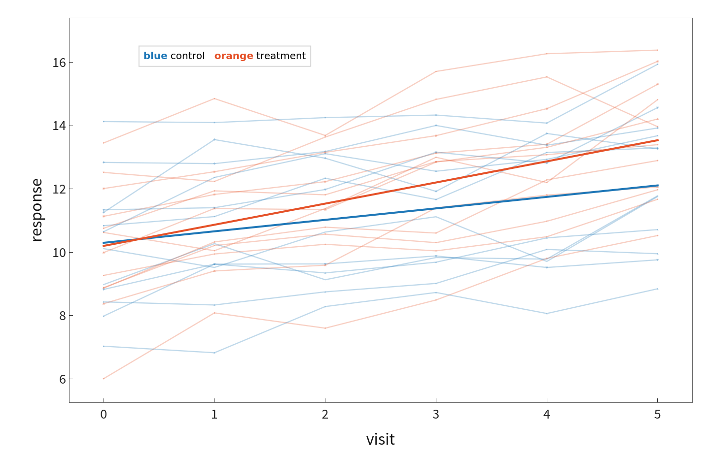
Thin lines are the 24 synthetic patients. Thick lines are the fitted population trajectories. The treatment contrast grows with visit rather than remaining constant.
1. The revised data-generating model
1. The revised data-generating model
y
ij
β
0
β
1
t
j
β
2
T
i
β
3
t
j
T
i
b
i
ϵ
ij
b
i
2
τ
ϵ
ij
2
σ
The residuals are independent conditional on the patient effect. Marginally, two observations from the same patient remain correlated because both contain b. Thus IID residuals do not mean independent repeated measurements.
BlockRandom[SeedRandom[6,Method"MersenneTwister"];patientIntercepts=RandomVariate[NormalDistribution[0.`,2.2`],24];iidErrors=RandomVariate[NormalDistribution[0.`,0.55`],{24,6}];];patientData=Flatten[Table[With[{tr=Boole[OddQ[i]]},Table[{N[t],tr,"P"<>IntegerString[i,10,2],N[10.`+0.35`t-0.2`tr+0.3`trt+patientIntercepts〚i〛+iidErrors〚i,t+1〛]},{t,0,5}]],{i,24}],1];
2. The interaction is an ordinary Wolfram expression
2. The interaction is an ordinary Wolfram expression
fit=MixedEffectsModelFit[patientData,{1,time,treatment,timetreatment},{{1},patient},{time,treatment,patient},Method"REML"];fit[{"FixedEffects","RandomEffectCovariances","ResidualVariance","Converged"}]
FixedEffects110.2988,time0.362358,treatment-0.0974337,time*treatment0.305073,RandomEffectCovariancespatient{{3.66801}},ResidualVariance0.335716,ConvergedTrue
The estimated interaction is 0.3051 response units per visit. It answers whether the two trajectories change at different rates. It is not itself the treatment difference at a particular visit. The table reports the Kenward-Roger small-sample result, independently matched to R's lmerTest/pbkrtest implementation.
estimand | estimate | SE | df | 95% interval | p-value |
time x treatment slope | 0.3051 | 0.0565 | 118.00 | 0.193, 0.417 | 3.58 x 10^-7 |
Visit-specific estimands
Visit-specific estimands
Δ(t)=+t=c(t)
β
2
β
3
β
c[t_]:={0.`,0.`,1.`,t};delta[t_]:=c[t].Values[fit["FixedEffects"]];se[t_]:=
c[t].fit["FixedEffectCovariance"].c[t]
;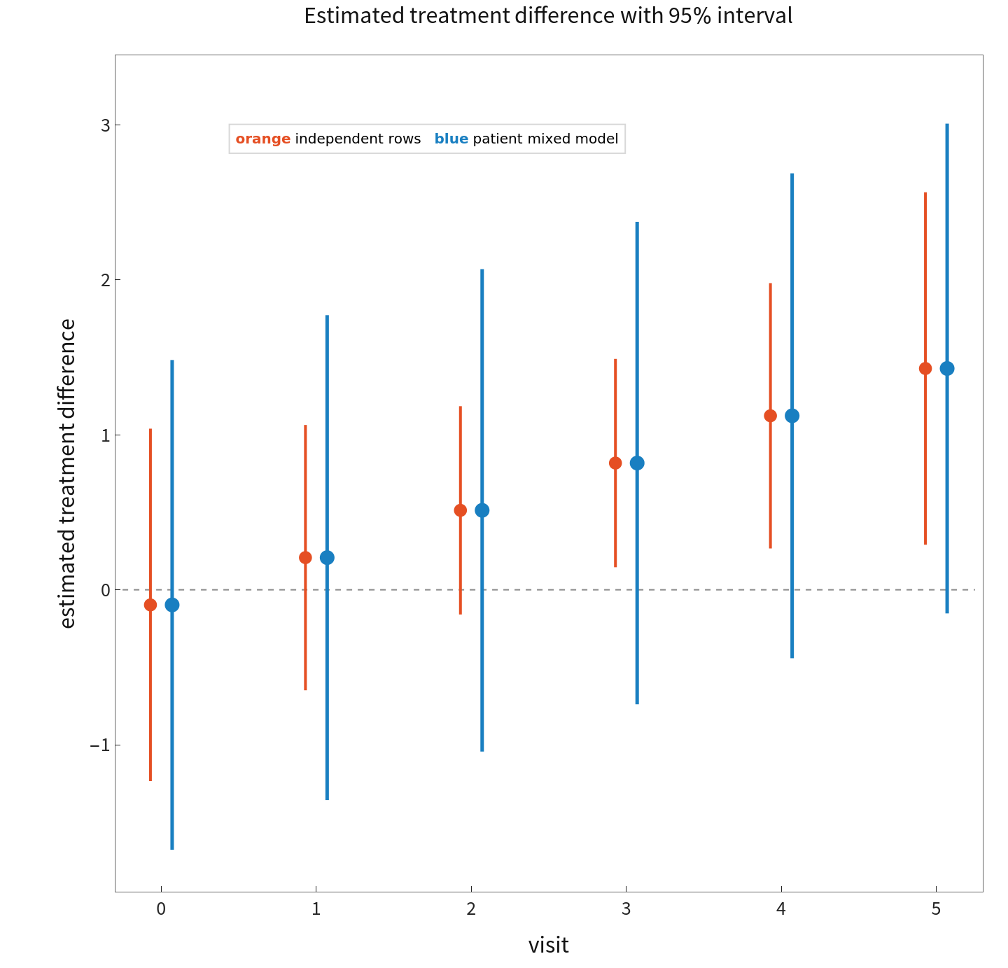
Both analyses estimate the same balanced-design mean trajectory. Their uncertainty differs because only the mixed model recognises 24 patients assigned at patient level rather than 144 independent experimental units.
3. The clinical question is a contrast, not one coefficient
3. The clinical question is a contrast, not one coefficient
For this illustration, define the final-visit treatment difference before looking at the fit. At visit 5 its estimate is 1.428. The invalid row-independent calculation reports p=0.013; the patient model reports p=0.074 with a normal Wald reference and p=0.087 with Kenward-Roger degrees of freedom. The interaction estimate is 0.305 (SE 0.057, 95% interval 0.193 to 0.417; p=3.58 x 10^-7). These are not contradictory results: one asks whether slopes differ, while the other asks whether the groups differ at a specified visit.
analysis and inference | visit-5 estimate | SE | 95% interval | p-value |
independent rows, normal Wald | 1.4279 | 0.5755 | 0.300, 2.556 | 0.0131 |
patient random intercept, normal Wald | 1.4279 | 0.8004 | -0.141, 2.997 | 0.0744 |
patient random intercept, Kenward-Roger | 1.4279 | 0.8004 | -0.226, 3.082 | 0.0874 |
Practical lesson. In a real protocol, pre-specify the visit or contrast that represents the clinical estimand. In this synthetic example, visit 5 is an explicitly defined illustrative estimand, not a claim of protocol pre-specification. Do not interpret the treatment main effect as an overall treatment effect when an interaction is present: here it is the treatment contrast at time zero.
4. Checked independently in R and Python
4. Checked independently in R and Python
The exact CSV generated above was refitted with current R lme4::lmer and Python's MixedLM. No reference result was copied into the Wolfram fitting function. The gate records the data MD5 and runtime/library versions, then checks all four fixed effects, the complete 4 by 4 fixed-effect covariance matrix, both variance components, the REML log likelihood, the interaction interval and p-value, and all six visit-specific contrasts and standard errors. A second gate checks Satterthwaite and Kenward-Roger estimates, standard errors, degrees of freedom, intervals, and p-values against R.
implementation | time x treatment | patient variance | residual variance | log likelihood | visit-5 SE | status |
Wolfram 15.0.1 for Mac OS X ARM (64-bit) (July 2, 2026) | 0.305073 | 3.668010 | 0.335716 | -178.049333 | 0.800402 | PASS |
R-lme4 2.0.1 | 0.305073 | 3.668011 | 0.335716 | -178.049333 | 0.800402 | PASS |
Python-statsmodels 0.14.5 | 0.305073 | 3.667989 | 0.335717 | -178.049333 | 0.800400 | PASS |
All 2 model comparisons and all 4 small-sample inference comparisons pass. The pass counts above are read from the comparison output; they are not hard-coded notebook claims.
5. From this demonstration to a trial analysis
5. From this demonstration to a trial analysis
The first two sensitivity checks are evaluated, not just recommended. The final-visit conclusion is shown under a patient random slope and under categorical visit indicators with treatment-by-visit interactions. All three native fits converge without a singularity warning.
sensitivity model | visit-5 estimate | SE | residual variance | converged | singular |
Linear visit + random intercept | 1.4279 | 0.8004 | 0.3357 | PASS | no |
Linear visit + random intercept and slope | 1.4279 | 0.7949 | 0.3265 | PASS | no |
Categorical visit + random intercept | 1.3130 | 0.8167 | 0.3341 | PASS | no |
Use categorical visit unless a linear trajectory is scientifically justified. Here the linear data-generating mechanism is known because the data are synthetic, so the linear model is the primary demonstration. A conventional trial MMRM often includes treatment, categorical visit, treatment-by-visit, and relevant baseline terms, with a pre-specified within-patient covariance. The compact random-intercept and random-slope analyses above are longitudinal LMMs; they should not be relabelled as a residual-only regulatory MMRM.
Check covariance sensitivity. The random-slope row is one such check. Depending on the design, defensible alternatives may also include AR(1), compound symmetry, or unstructured residual covariance. Choose them from the design and a pre-specified analysis plan, not by searching for the smallest p-value.
Handle inference and missingness explicitly. The tables above now use explicit normal-Wald and Kenward-Roger labels. A trial report should also state confidence intervals, convergence and singularity diagnostics, missing-row handling, and the assumption under which incomplete outcomes are analysed.
Separate three questions. The interaction, each visit-specific contrast, and a global treatment hypothesis are different estimands. A useful report states which one drives the decision and why.
6. Reproduce the check
6. Reproduce the check
Clone or download the public repository and open this notebook inside its Community folder. The package itself has no R, Python, API, or network dependency. Those programs are used only to repeat the independent validation.
repoRoot=DirectoryName[NotebookDirectory[]];validationDir=FileNameJoin[{repoRoot,"Validation"}];pythonCandidates=DeleteDuplicates[Select[{Environment["MMAMIXEDEFFECTS_PYTHON"],FileNameJoin[{$HomeDirectory,"anaconda3","bin","python3"}],FindExecutable["python3"],FindExecutable["python"]},StringQ]];scientificPython=SelectFirst[pythonCandidates,RunProcess[{#1,"-c","import numpy,pandas,scipy,statsmodels"}]["ExitCode"]0&,Missing["NoScientificPython"]];
rRun=RunProcess[{FindExecutable["Rscript"],FileNameJoin[{validationDir,"RunTreatmentTimeRReference.R"}]}];pythonRun=RunProcess[{scientificPython,FileNameJoin[{validationDir,"RunTreatmentTimePythonReference.py"}]}];wlRun=RunProcess[{FindExecutable["wolframscript"],"-file",FileNameJoin[{validationDir,"RunTreatmentTimeWolframReference.wls"}]}];gateRun=RunProcess[{scientificPython,FileNameJoin[{validationDir,"CompareTreatmentTimeReferences.py"}]}];Association["R"rRun["ExitCode"],"Python"pythonRun["ExitCode"],"Wolfram"wlRun["ExitCode"],"Gate"gateRun["ExitCode"]]