Visualizing the Gradient Vector

function

maximum

minimum

linear

saddle 1

saddle 2

example 1

example 2

location

The gradient vector

∇f(x,y)

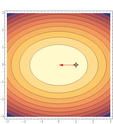
evaluated at a point

(a,b)

is superimposed on a contour plot of the function

f(x,y)

. By moving the point

(a,b)

around the plot region, you can see how the magnitude and direction of the gradient vector change. You can normalize the gradient vector to focus only on its direction, which is particularly useful where its magnitude is very small.

Coordinates of the point in the plot region can be viewed by hovering the mouse over the point. Components of the vectors

∇f

and

-∇f

can viewed by hovering the mouse over the vectors.

Permanent Citation

Eric Schulz

"Visualizing the Gradient Vector"
http://demonstrations.wolfram.com/VisualizingTheGradientVector/
Wolfram Demonstrations Project
Published: September 28, 2007